GiNaC 
This is a tutorial that documents GiNaC 1.8.10, an open framework for symbolic computation within the C++ programming language.
Table of Contents
- 1 Introduction
- 2 A Tour of GiNaC
- 3 Installation
- 4 Basic concepts
- 4.1 Expressions
- 4.2 Automatic evaluation and canonicalization of expressions
- 4.3 Error handling
- 4.4 The class hierarchy
- 4.5 Symbols
- 4.6 Numbers
- 4.7 Constants
- 4.8 Sums, products and powers
- 4.9 Lists of expressions
- 4.10 Mathematical functions
- 4.11 Relations
- 4.12 Integrals
- 4.13 Matrices
- 4.14 Indexed objects
- 4.15 Non-commutative objects
- 5 Methods and functions
- 5.1 Getting information about expressions
- 5.2 Numerical evaluation
- 5.3 Substituting expressions
- 5.4 Pattern matching and advanced substitutions
- 5.5 Applying a function on subexpressions
- 5.6 Visitors and tree traversal
- 5.7 Polynomial arithmetic
- 5.7.1 Testing whether an expression is a polynomial
- 5.7.2 Expanding and collecting
- 5.7.3 Degree and coefficients
- 5.7.4 Polynomial division
- 5.7.5 Unit, content and primitive part
- 5.7.6 GCD, LCM and resultant
- 5.7.7 Square-free decomposition
- 5.7.8 Square-free partial fraction decomposition
- 5.7.9 Polynomial factorization
- 5.8 Rational expressions
- 5.9 Symbolic differentiation
- 5.10 Series expansion
- 5.11 Symmetrization
- 5.12 Predefined mathematical functions
- 5.13 Complex expressions
- 5.14 Solving linear systems of equations
- 5.15 Input and output of expressions
- 6 Extending GiNaC
- 7 A Comparison With Other CAS
- Appendix A Internal structures
- Appendix B Package tools
- Appendix C Bibliography
- Concept index
1 Introduction 
The motivation behind GiNaC derives from the observation that most present day computer algebra systems (CAS) are linguistically and semantically impoverished. Although they are quite powerful tools for learning math and solving particular problems they lack modern linguistic structures that allow for the creation of large-scale projects. GiNaC is an attempt to overcome this situation by extending a well established and standardized computer language (C++) by some fundamental symbolic capabilities, thus allowing for integrated systems that embed symbolic manipulations together with more established areas of computer science (like computation-intense numeric applications, graphical interfaces, etc.) under one roof.
The particular problem that led to the writing of the GiNaC framework is still a very active field of research, namely the calculation of higher order corrections to elementary particle interactions. There, theoretical physicists are interested in matching present day theories against experiments taking place at particle accelerators. The computations involved are so complex they call for a combined symbolical and numerical approach. This turned out to be quite difficult to accomplish with the present day CAS we have worked with so far and so we tried to fill the gap by writing GiNaC. But of course its applications are in no way restricted to theoretical physics.
This tutorial is intended for the novice user who is new to GiNaC but already has some background in C++ programming. However, since a hand-made documentation like this one is difficult to keep in sync with the development, the actual documentation is inside the sources in the form of comments. That documentation may be parsed by one of the many Javadoc-like documentation systems. If you fail at generating it you may access it from the GiNaC home page. It is an invaluable resource not only for the advanced user who wishes to extend the system (or chase bugs) but for everybody who wants to comprehend the inner workings of GiNaC. This little tutorial on the other hand only covers the basic things that are unlikely to change in the near future.
1.1 License 
The GiNaC framework for symbolic computation within the C++ programming language is Copyright © 1999-2026 Johannes Gutenberg University Mainz, Germany.
This program is free software; you can redistribute it and/or modify it under the terms of the GNU General Public License as published by the Free Software Foundation; either version 2 of the License, or (at your option) any later version.
This program is distributed in the hope that it will be useful, but WITHOUT ANY WARRANTY; without even the implied warranty of MERCHANTABILITY or FITNESS FOR A PARTICULAR PURPOSE. See the GNU General Public License for more details.
You should have received a copy of the GNU General Public License along with this program; see the file COPYING. If not, see https://www.gnu.org/licenses/.
2 A Tour of GiNaC 
This quick tour of GiNaC wants to arise your interest in the subsequent chapters by showing off a bit. Please excuse us if it leaves many open questions.
2.1 How to use it from within C++ 
The GiNaC open framework for symbolic computation within the C++ programming language does not try to define a language of its own as conventional CAS do. Instead, it extends the capabilities of C++ by symbolic manipulations. Here is how to generate and print a simple (and rather pointless) bivariate polynomial with some large coefficients:
#include <iostream>
#include <ginac/ginac.h>
using namespace std;
using namespace GiNaC;

int main()
{
    symbol x("x"), y("y");
    ex poly;

    for (int i=0; i<3; ++i)
        poly += factorial(i+16)*pow(x,i)*pow(y,2-i);

    cout << poly << endl;
    return 0;
}
Assuming the file is called hello.cc, on our system we can compile and run it like this:
$ c++ hello.cc -o hello -lginac -lcln
$ ./hello
355687428096000*x*y+20922789888000*y^2+6402373705728000*x^2
(See Package tools, for tools that help you when creating a software package that uses GiNaC.)
Next, there is a more meaningful C++ program that calls a function which generates Hermite polynomials in a specified free variable.
#include <iostream>
#include <ginac/ginac.h>
using namespace std;
using namespace GiNaC;

ex HermitePoly(const symbol & x, int n)
{
    ex HKer=exp(-pow(x, 2));
    // uses the identity H_n(x) == (-1)^n exp(x^2) (d/dx)^n exp(-x^2)
    return normal(pow(-1, n) * diff(HKer, x, n) / HKer);
}

int main()
{
    symbol z("z");

    for (int i=0; i<6; ++i)
        cout << "H_" << i << "(z) == " << HermitePoly(z,i) << endl;

    return 0;
}
When run, this will type out
H_0(z) == 1
H_1(z) == 2*z
H_2(z) == 4*z^2-2
H_3(z) == -12*z+8*z^3
H_4(z) == -48*z^2+16*z^4+12
H_5(z) == 120*z-160*z^3+32*z^5
This method of generating the coefficients is of course far from optimal for production purposes.
In order to show some more examples of what GiNaC can do we will now use
the ginsh, a simple GiNaC interactive shell that provides a
convenient window into GiNaC’s capabilities.
2.2 What it can do for you 
After invoking ginsh one can test and experiment with GiNaC’s
features much like in other Computer Algebra Systems except that it does
not provide programming constructs like loops or conditionals. For a
concise description of the ginsh syntax we refer to its
accompanied man page. Suffice to say that assignments and comparisons in
ginsh are written as they are in C, i.e. = assigns and
== compares.
It can manipulate arbitrary precision integers in a very fast way. Rational numbers are automatically converted to fractions of coprime integers:
> x=3^150;
369988485035126972924700782451696644186473100389722973815184405301748249
> y=3^149;
123329495011708990974900260817232214728824366796574324605061468433916083
> x/y;
3
> y/x;
1/3
Exact numbers are always retained as exact numbers and only evaluated as floating point numbers if requested. For instance, with numeric radicals is dealt pretty much as with symbols. Products of sums of them can be expanded:
> expand((1+a^(1/5)-a^(2/5))^3);
1+3*a+3*a^(1/5)-5*a^(3/5)-a^(6/5)
> expand((1+3^(1/5)-3^(2/5))^3);
10-5*3^(3/5)
> evalf((1+3^(1/5)-3^(2/5))^3);
0.33408977534118624228
The function evalf that was used above converts any number in
GiNaC’s expressions into floating point numbers. This can be done to
arbitrary predefined accuracy:
> evalf(1/7);
0.14285714285714285714
> Digits=150;
150
> evalf(1/7);
0.1428571428571428571428571428571428571428571428571428571428571428571428
5714285714285714285714285714285714285
Exact numbers other than rationals that can be manipulated in GiNaC
include predefined constants like Archimedes’ Pi. They can both
be used in symbolic manipulations (as an exact number) as well as in
numeric expressions (as an inexact number):
> a=Pi^2+x;
x+Pi^2
> evalf(a);
9.869604401089358619+x
> x=2;
2
> evalf(a);
11.869604401089358619
Built-in functions evaluate immediately to exact numbers if this is possible. Conversions that can be safely performed are done immediately; conversions that are not generally valid are not done:
> cos(42*Pi);
1
> cos(acos(x));
x
> acos(cos(x));
acos(cos(x))
(Note that converting the last input to x would allow one to
conclude that 42*Pi is equal to 0.)
Linear equation systems can be solved along with basic linear
algebra manipulations over symbolic expressions. In C++ GiNaC offers
a matrix class for this purpose but we can see what it can do using
ginsh’s bracket notation to type them in:
> lsolve(a+x*y==z,x);
y^(-1)*(z-a);
> lsolve({3*x+5*y == 7, -2*x+10*y == -5}, {x, y});
{x==19/8,y==-1/40}
> M = [ [1, 3], [-3, 2] ];
[[1,3],[-3,2]]
> determinant(M);
11
> charpoly(M,lambda);
lambda^2-3*lambda+11
> A = [ [1, 1], [2, -1] ];
[[1,1],[2,-1]]
> A+2*M;
[[1,1],[2,-1]]+2*[[1,3],[-3,2]]
> evalm(%);
[[3,7],[-4,3]]
> B = [ [0, 0, a], [b, 1, -b], [-1/a, 0, 0] ];
> evalm(B^(2^12345));
[[1,0,0],[0,1,0],[0,0,1]]
Multivariate polynomials and rational functions may be expanded, collected, factorized, and normalized (i.e. converted to a ratio of two coprime polynomials):
> a = x^4 + 2*x^2*y^2 + 4*x^3*y + 12*x*y^3 - 3*y^4;
12*x*y^3+2*x^2*y^2+4*x^3*y-3*y^4+x^4
> b = x^2 + 4*x*y - y^2;
4*x*y-y^2+x^2
> expand(a*b);
8*x^5*y+17*x^4*y^2+43*x^2*y^4-24*x*y^5+16*x^3*y^3+3*y^6+x^6
> factor(%);
(4*x*y+x^2-y^2)^2*(x^2+3*y^2)
> collect(a+b,x);
4*x^3*y-y^2-3*y^4+(12*y^3+4*y)*x+x^4+x^2*(1+2*y^2)
> collect(a+b,y);
12*x*y^3-3*y^4+(-1+2*x^2)*y^2+(4*x+4*x^3)*y+x^2+x^4
> normal(a/b);
3*y^2+x^2
Here we have made use of the ginsh-command % to pop the
previously evaluated element from ginsh’s internal stack.
You can differentiate functions and expand them as Taylor or Laurent
series in a very natural syntax (the second argument of series is
a relation defining the evaluation point, the third specifies the
order):
> diff(tan(x),x);
tan(x)^2+1
> series(sin(x),x==0,4);
x-1/6*x^3+Order(x^4)
> series(1/tan(x),x==0,4);
x^(-1)-1/3*x-1/45*x^3+Order(x^4)
> series(tgamma(x),x==0,3);
x^(-1)-Euler+(1/12*Pi^2+1/2*Euler^2)*x+
(-1/3*zeta(3)-1/12*Pi^2*Euler-1/6*Euler^3)*x^2+Order(x^3)
> evalf(%);
x^(-1)-0.5772156649015328606+(0.9890559953279725555)*x
-(0.90747907608088628905)*x^2+Order(x^3)
> series(tgamma(2*sin(x)-2),x==Pi/2,6);
-(x-1/2*Pi)^(-2)+(-1/12*Pi^2-1/2*Euler^2-1/240)*(x-1/2*Pi)^2
-Euler-1/12+Order((x-1/2*Pi)^3)
Often, functions don’t have roots in closed form. Nevertheless, it’s quite easy to compute a solution numerically, to arbitrary precision:
> Digits=50:
> fsolve(cos(x)==x,x,0,2);
0.7390851332151606416553120876738734040134117589007574649658
> f=exp(sin(x))-x:
> X=fsolve(f,x,-10,10);
2.2191071489137460325957851882042901681753665565320678854155
> subs(f,x==X);
-6.372367644529809108115521591070847222364418220770475144296E-58
Notice how the final result above differs slightly from zero by about
6*10^(-58). This is because with 50 decimal digits precision the
root cannot be represented more accurately than X. Such
inaccuracies are to be expected when computing with finite floating
point values.
If you ever wanted to convert units in C or C++ and found this is cumbersome, here is the solution. Symbolic types can always be used as tags for different types of objects. Converting from wrong units to the metric system is now easy:
> in=.0254*m;
0.0254*m
> lb=.45359237*kg;
0.45359237*kg
> 200*lb/in^2;
140613.91592783185568*kg*m^(-2)
3 Installation 
GiNaC’s installation follows the spirit of most GNU software. It is easily installed on your system by three steps: configuration, build, installation.
3.1 Prerequisites 
In order to install GiNaC on your system, some prerequisites need to be
met. First of all, you need to have a C++-compiler adhering to the
ISO standard ISO/IEC 14882:2014(E). We used GCC for development
so if you have a different compiler you are on your own. For the
configuration to succeed you need a Posix compliant shell installed in
/bin/sh, GNU bash is fine. The pkgconf utility is
required for the configuration, it can be downloaded from
http://pkgconf.org/. Last but not least, the CLN library
is used extensively and needs to be installed on your system.
Please get it from https://www.ginac.de/CLN/ (it is licensed under
the GPL) and install it prior to trying to install GiNaC. The configure
script checks if it can find it and if it cannot, it will refuse to
continue.
3.2 Configuration 
To configure GiNaC means to prepare the source distribution for
building. It is done via a shell script called configure that
is shipped with the sources and was originally generated by GNU
Autoconf. Since a configure script generated by GNU Autoconf never
prompts, all customization must be done either via command line
parameters or environment variables. It accepts a list of parameters,
the complete set of which can be listed by calling it with the
--help option. The most important ones will be shortly
described in what follows:
- --disable-shared: When given, this option switches off the build of a shared library, i.e. a .so file. This may be convenient when developing because it considerably speeds up compilation.
- --prefix=PREFIX: The directory where the compiled library and headers are installed. It defaults to /usr/local which means that the library is installed in the directory /usr/local/lib, the header files in /usr/local/include/ginac and the documentation (like this one) into /usr/local/share/doc/GiNaC.
- --libdir=LIBDIR: Use this option in case you want to have the library installed in some other directory than PREFIX/lib/.
- --includedir=INCLUDEDIR: Use this option in case you want to have the header files installed in some other directory than PREFIX/include/ginac/. For instance, if you specify --includedir=/usr/include you will end up with the header files sitting in the directory /usr/include/ginac/. Note that the subdirectory ginac is enforced by this process in order to keep the header files separated from others. This avoids some clashes and allows for an easier deinstallation of GiNaC. This ought to be considered A Good Thing (tm).
- --datadir=DATADIR: This option may be given in case you want to have the documentation installed in some other directory than PREFIX/share/doc/GiNaC/.
In addition, you may specify some environment variables. CXX
holds the path and the name of the C++ compiler in case you want to
override the default in your path. (The configure script
searches your path for g++, c++, aCC,
cxx, cc++, clang++, in that order.) It may
be very useful to define some compiler flags with the CXXFLAGS
environment variable, like optimization, debugging information and
warning levels. If omitted, it defaults to -g
-O2.1
The whole process is illustrated in the following two
examples. (Substitute setenv VARIABLE value for
export VARIABLE=value if the Berkeley C shell is
your login shell.)
Here is a simple configuration for a site-wide GiNaC library assuming everything is in default paths:
$ export CXXFLAGS="-Wall -O2"
$ ./configure
And here is a configuration for a private static GiNaC library with several components sitting in custom places (site-wide GCC and private CLN). The compiler is persuaded to be picky and full assertions and debugging information are switched on:
$ export CXX=/usr/local/gnu/bin/c++
$ export CPPFLAGS="$(CPPFLAGS) -I$(HOME)/include"
$ export CXXFLAGS="$(CXXFLAGS) -DDO_GINAC_ASSERT -ggdb -Wall -pedantic"
$ export LDFLAGS="$(LDFLAGS) -L$(HOME)/lib"
$ ./configure --disable-shared --prefix=$(HOME)
3.3 Building GiNaC 
After proper configuration you should just build the whole library by typing
$ make
at the command prompt and go for a cup of coffee. The exact time it
takes to compile GiNaC depends not only on the speed of your machines
but also on other parameters, for instance what value for CXXFLAGS
you entered. Optimization may be very time-consuming.
Just to make sure GiNaC works properly you may run a collection of regression tests by typing
$ make check
This will compile some sample programs, run them and check the output for correctness. The regression tests fall in three categories. First, the so called exams are performed, simple tests where some predefined input is evaluated (like a pupils’ exam). Second, the checks test the coherence of results among each other with possible random input. Third, some timings are performed, which benchmark some predefined problems with different sizes and display the CPU time used in seconds. Each individual test should return a message ‘passed’. This is mostly intended to be a QA-check if something was broken during development, not a sanity check of your system. Some of the tests in sections checks and timings may require insane amounts of memory and CPU time. Feel free to kill them if your machine catches fire. Another quite important intent is to allow people to fiddle around with optimization.
By default, the only documentation that will be built is this tutorial in .info format. To build the GiNaC tutorial and reference manual in HTML, DVI, PostScript, or PDF formats, use one of
$ make html
$ make dvi
$ make ps
$ make pdf
Generally, the top-level Makefile runs recursively to the
subdirectories. It is therefore safe to go into any subdirectory
(doc/, ginsh/, …) and simply type make
target there in case something went wrong.
3.4 Installing GiNaC 
To install GiNaC on your system, simply type
$ make install
As described in the section about configuration the files will be installed in the following directories (the directories will be created if they don’t already exist):
- libginac.a will go into PREFIX/lib/ (or LIBDIR if specified) which defaults to /usr/local/lib/. So will libginac.so unless the configure script was given the option --disable-shared. The proper symlinks will be established as well.
- All the header files will be installed into PREFIX/include/ginac/ (or INCLUDEDIR/ginac/, if specified).
- All documentation (info) will be stuffed into PREFIX/share/doc/GiNaC/ (or DATADIR/doc/GiNaC/, if DATADIR was specified).
For the sake of completeness we will list some other useful make
targets: make clean deletes all files generated by
make, i.e. all the object files. In addition make
distclean removes all files generated by the configuration and
make maintainer-clean goes one step further and deletes files
that may require special tools to rebuild (like the libtool
for instance). Finally make uninstall removes the installed
library, header files and documentation2.
4 Basic concepts 
This chapter will describe the different fundamental objects that can be handled by GiNaC. But before doing so, it is worthwhile introducing you to the more commonly used class of expressions, representing a flexible meta-class for storing all mathematical objects.
- Expressions
- Automatic evaluation and canonicalization of expressions
- Error handling
- The class hierarchy
- Symbols
- Numbers
- Constants
- Sums, products and powers
- Lists of expressions
- Mathematical functions
- Relations
- Integrals
- Matrices
- Indexed objects
- Non-commutative objects
4.1 Expressions 
The most common class of objects a user deals with is the expression
ex, representing a mathematical object like a variable, number,
function, sum, product, etc… Expressions may be put together to form
new expressions, passed as arguments to functions, and so on. Here is a
little collection of valid expressions:
ex MyEx1 = 5;                       // simple number
ex MyEx2 = x + 2*y;                 // polynomial in x and y
ex MyEx3 = (x + 1)/(x - 1);         // rational expression
ex MyEx4 = sin(x + 2*y) + 3*z + 41; // containing a function
ex MyEx5 = MyEx4 + 1;               // similar to above
Expressions are handles to other more fundamental objects, that often
contain other expressions thus creating a tree of expressions
(See Internal structures, for particular examples). Most methods on
ex therefore run top-down through such an expression tree. For
example, the method has() scans recursively for occurrences of
something inside an expression. Thus, if you have declared MyEx4
as in the example above MyEx4.has(y) will find y inside
the argument of sin and hence return true.
The next sections will outline the general picture of GiNaC’s class
hierarchy and describe the classes of objects that are handled by
ex.
4.1.1 Note: Expressions and STL containers 
GiNaC expressions (ex objects) have value semantics (they can be
assigned, reassigned and copied like integral types) but the operator
< doesn’t provide a well-defined ordering on them. In STL-speak,
expressions are ‘Assignable’ but not ‘LessThanComparable’.
This implies that in order to use expressions in sorted containers such as
std::map<> and std::set<> you have to supply a suitable
comparison predicate. GiNaC provides such a predicate, called
ex_is_less. For example, a set of expressions should be defined
as std::set<ex, ex_is_less>.
Unsorted containers such as std::vector<> and std::list<>
don’t pose a problem. A std::vector<ex> works as expected.
See Getting information about expressions, for more about comparing and ordering expressions.
4.2 Automatic evaluation and canonicalization of expressions 
GiNaC performs some automatic transformations on expressions, to simplify them and put them into a canonical form. Some examples:
ex MyEx1 = 2*x - 1 + x;  // 3*x-1
ex MyEx2 = x - x;        // 0
ex MyEx3 = cos(2*Pi);    // 1
ex MyEx4 = x*y/x;        // y
This behavior is usually referred to as automatic or anonymous evaluation. GiNaC only performs transformations that are
- at most of complexity O(n log n)
- algebraically correct, possibly except for a set of measure zero (e.g. x/x is transformed to 1 although this is incorrect for x=0)
There are two types of automatic transformations in GiNaC that may not behave in an entirely obvious way at first glance:
- The terms of sums and products (and some other things like the arguments of symmetric functions, the indices of symmetric tensors etc.) are re-ordered into a canonical form that is deterministic, but not lexicographical or in any other way easy to guess (it almost always depends on the number and order of the symbols you define). However, constructing the same expression twice, either implicitly or explicitly, will always result in the same canonical form.
- Expressions of the form ’number times sum’ are automatically expanded (this
has to do with GiNaC’s internal representation of sums and products). For
example
ex MyEx5 = 2*(x + y);   // 2*x+2*y
ex MyEx6 = z*(x + y);   // z*(x+y)
The general rule is that when you construct expressions, GiNaC automatically creates them in canonical form, which might differ from the form you typed in your program. This may create some awkward looking output (‘-y+x’ instead of ‘x-y’) but allows for more efficient operation and usually yields some immediate simplifications.
Internally, the anonymous evaluator in GiNaC is implemented by the methods
ex ex::eval() const;
ex basic::eval() const;
but unless you are extending GiNaC with your own classes or functions, there
should never be any reason to call them explicitly. All GiNaC methods that
transform expressions, like subs() or normal(), automatically
re-evaluate their results.
4.3 Error handling 
GiNaC reports run-time errors by throwing C++ exceptions. All exceptions
generated by GiNaC are subclassed from the standard exception class
defined in the <stdexcept> header. In addition to the predefined
logic_error, domain_error, out_of_range,
invalid_argument, runtime_error, range_error and
overflow_error types, GiNaC also defines a pole_error
exception that gets thrown when trying to evaluate a mathematical function
at a singularity.
The pole_error class has a member function
int pole_error::degree() const;
that returns the order of the singularity (or 0 when the pole is logarithmic or the order is undefined).
When using GiNaC it is useful to arrange for exceptions to be caught in the main program even if you don’t want to do any special error handling. Otherwise whenever an error occurs in GiNaC, it will be delegated to the default exception handler of your C++ compiler’s run-time system which usually only aborts the program without giving any information what went wrong.
Here is an example for a main() function that catches and prints
exceptions generated by GiNaC:
#include <iostream>
#include <stdexcept>
#include <ginac/ginac.h>
using namespace std;
using namespace GiNaC;

int main()
{
    try {
        ...
        // code using GiNaC
        ...
    } catch (exception &p) {
        cerr << p.what() << endl;
        return 1;
    }
    return 0;
}
4.4 The class hierarchy 
GiNaC’s class hierarchy consists of several classes representing
mathematical objects, all of which (except for ex and some
helpers) are internally derived from one abstract base class called
basic. You do not have to deal with objects of class
basic, instead you’ll be dealing with symbols, numbers,
containers of expressions and so on.
To get an idea about what kinds of symbolic composites may be built we have a look at the most important classes in the class hierarchy and some of the relations among the classes:
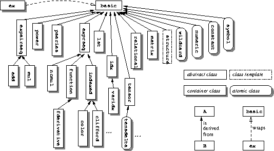
The abstract classes shown here (the ones without drop-shadow) are of no
interest for the user. They are used internally in order to avoid code
duplication if two or more classes derived from them share certain
features. An example is expairseq, a container for a sequence of
pairs each consisting of one expression and a number (numeric).
What is visible to the user are the derived classes add
and mul, representing sums and products. See Internal structures, where these two classes are described in more detail. The
following table shortly summarizes what kinds of mathematical objects
are stored in the different classes:
|
4.5 Symbols 
Symbolic indeterminates, or symbols for short, are for symbolic manipulation what atoms are for chemistry.
A typical symbol definition looks like this:
symbol x("x");
This definition actually contains three very different things:
- a C++ variable named
x - a
symbolobject stored in this C++ variable; this object represents the symbol in a GiNaC expression - the string
"x"which is the name of the symbol, used (almost) exclusively for printing expressions holding the symbol
Symbols have an explicit name, supplied as a string during construction, because in C++, variable names can’t be used as values, and the C++ compiler throws them away during compilation.
It is possible to omit the symbol name in the definition:
symbol x;
In this case, GiNaC will assign the symbol an internal, unique name of the
form symbolNNN. This won’t affect the usability of the symbol but
the output of your calculations will become more readable if you give your
symbols sensible names (for intermediate expressions that are only used
internally such anonymous symbols can be quite useful, however).
Now, here is one important property of GiNaC that differentiates it from
other computer algebra programs you may have used: GiNaC does not use
the names of symbols to tell them apart, but a (hidden) serial number that
is unique for each newly created symbol object. If you want to use
one and the same symbol in different places in your program, you must only
create one symbol object and pass that around. If you create another
symbol, even if it has the same name, GiNaC will treat it as a different
indeterminate.
Observe:
ex f(int n)
{
    symbol x("x");
    return pow(x, n);
}

int main()
{
    symbol x("x");
    ex e = f(6);

    cout << e << endl;
     // prints "x^6" which looks right, but...

    cout << e.degree(x) << endl;
     // ...this doesn't work. The symbol "x" here is different from the one
     // in f() and in the expression returned by f(). Consequently, it
     // prints "0".
}
One possibility to ensure that f() and main() use the same
symbol is to pass the symbol as an argument to f():
ex f(int n, const ex & x)
{
    return pow(x, n);
}

int main()
{
    symbol x("x");

    // Now, f() uses the same symbol.
    ex e = f(6, x);

    cout << e.degree(x) << endl;
     // prints "6", as expected
}
Another possibility would be to define a global symbol x that is used
by both f() and main(). If you are using global symbols and
multiple compilation units you must take special care, however. Suppose
that you have a header file globals.h in your program that defines
a symbol x("x");. In this case, every unit that includes
globals.h would also get its own definition of x (because
header files are just inlined into the source code by the C++ preprocessor),
and hence you would again end up with multiple equally-named, but different,
symbols. Instead, the globals.h header should only contain a
declaration like extern symbol x;, with the definition of
x moved into a C++ source file such as globals.cpp.
A different approach to ensuring that symbols used in different parts of your program are identical is to create them with a factory function like this one:
const symbol & get_symbol(const string & s)
{
    static map<string, symbol> directory;
    map<string, symbol>::iterator i = directory.find(s);
    if (i != directory.end())
        return i->second;
    else
        return directory.insert(make_pair(s, symbol(s))).first->second;
}
This function returns one newly constructed symbol for each name that is passed in, and it returns the same symbol when called multiple times with the same name. Using this symbol factory, we can rewrite our example like this:
ex f(int n)
{
    return pow(get_symbol("x"), n);
}

int main()
{
    ex e = f(6);

    // Both calls of get_symbol("x") yield the same symbol.
    cout << e.degree(get_symbol("x")) << endl;
     // prints "6"
}
Instead of creating symbols from strings we could also have
get_symbol() take, for example, an integer number as its argument.
In this case, we would probably want to give the generated symbols names
that include this number, which can be accomplished with the help of an
ostringstream.
In general, if you’re getting weird results from GiNaC such as an expression ‘x-x’ that is not simplified to zero, you should check your symbol definitions.
As we said, the names of symbols primarily serve for purposes of expression output. But there are actually two instances where GiNaC uses the names for identifying symbols: When constructing an expression from a string, and when recreating an expression from an archive (see Input and output of expressions).
In addition to its name, a symbol may contain a special string that is used in LaTeX output:
symbol x("x", "\\Box");
This creates a symbol that is printed as "x" in normal output, but
as "\Box" in LaTeX code (See Input and output of expressions, for more
information about the different output formats of expressions in GiNaC).
GiNaC automatically creates proper LaTeX code for symbols having names of
greek letters (‘alpha’, ‘mu’, etc.). You can retrieve the name
and the LaTeX name of a symbol using the respective methods:
symbol::get_name() const;
symbol::get_TeX_name() const;
Symbols in GiNaC can’t be assigned values. If you need to store results of
calculations and give them a name, use C++ variables of type ex.
If you want to replace a symbol in an expression with something else, you
can invoke the expression’s .subs() method
(see Substituting expressions).
By default, symbols are expected to stand in for complex values, i.e. they live
in the complex domain. As a consequence, operations like complex conjugation,
for example (see Complex expressions), do not evaluate if applied
to such symbols. Likewise log(exp(x)) does not evaluate to x,
because of the unknown imaginary part of x.
On the other hand, if you are sure that your symbols will hold only real
values, you would like to have such functions evaluated. Therefore GiNaC
allows you to specify
the domain of the symbol. Instead of symbol x("x"); you can write
realsymbol x("x"); to tell GiNaC that x stands in for real values.
Furthermore, it is also possible to declare a symbol as positive. This will,
for instance, enable the automatic simplification of abs(x) into
x. This is done by declaring the symbol as possymbol x("x");.
4.6 Numbers 
For storing numerical things, GiNaC uses Bruno Haible’s library CLN. The classes therein serve as foundation classes for GiNaC. CLN stands for Class Library for Numbers or alternatively for Common Lisp Numbers. In order to find out more about CLN’s internals, the reader is referred to the documentation of that library. See The CLN Manual, for more information. Suffice to say that it is by itself build on top of another library, the GNU Multiple Precision library GMP, which is an extremely fast library for arbitrary long integers and rationals as well as arbitrary precision floating point numbers. It is very commonly used by several popular cryptographic applications. CLN extends GMP by several useful things: First, it introduces the complex number field over either reals (i.e. floating point numbers with arbitrary precision) or rationals. Second, it automatically converts rationals to integers if the denominator is unity and complex numbers to real numbers if the imaginary part vanishes and also correctly treats algebraic functions. Third it provides good implementations of state-of-the-art algorithms for all trigonometric and hyperbolic functions as well as for calculation of some useful constants.
The user can construct an object of class numeric in several
ways. The following example shows the four most important constructors.
It uses construction from C-integer, construction of fractions from two
integers, construction from C-float and construction from a string:
#include <iostream>
#include <ginac/ginac.h>
using namespace GiNaC;

int main()
{
    numeric two = 2;                      // exact integer 2
    numeric r(2,3);                       // exact fraction 2/3
    numeric e(2.71828);                   // floating point number
    numeric p = "3.14159265358979323846"; // constructor from string
    // Trott's constant in scientific notation:
    numeric trott("1.0841015122311136151E-2");

    std::cout << two*p << std::endl;  // floating point 6.283...
    ...
The imaginary unit in GiNaC is a predefined numeric object with the
name I:
    ...
    numeric z1 = 2-3*I;                    // exact complex number 2-3i
    numeric z2 = 5.9+1.6*I;                // complex floating point number
}
It may be tempting to construct fractions by writing numeric r(3/2).
This would, however, call C’s built-in operator / for integers
first and result in a numeric holding a plain integer 1. Never
use the operator / on integers unless you know exactly what you
are doing! Use the constructor from two integers instead, as shown in
the example above. Writing numeric(1)/2 may look funny but works
also.
We have seen now the distinction between exact numbers and floating
point numbers. Clearly, the user should never have to worry about
dynamically created exact numbers, since their ‘exactness’ always
determines how they ought to be handled, i.e. how ‘long’ they are. The
situation is different for floating point numbers. Their accuracy is
controlled by one global variable, called Digits. (For
those readers who know about Maple: it behaves very much like Maple’s
Digits). All objects of class numeric that are constructed from
then on will be stored with a precision matching that number of decimal
digits:
#include <iostream>
#include <ginac/ginac.h>
using namespace std;
using namespace GiNaC;

void foo()
{
    numeric three(3.0), one(1.0);
    numeric x = one/three;

    cout << "in " << Digits << " digits:" << endl;
    cout << x << endl;
    cout << Pi.evalf() << endl;
}

int main()
{
    foo();
    Digits = 60;
    foo();
    return 0;
}
The above example prints the following output to screen:
in 17 digits:
0.33333333333333333334
3.1415926535897932385
in 60 digits:
0.33333333333333333333333333333333333333333333333333333333333333333334
3.1415926535897932384626433832795028841971693993751058209749445923078
Note that the last number is not necessarily rounded as you would naively expect it to be rounded in the decimal system. But note also, that in both cases you got a couple of extra digits. This is because numbers are internally stored by CLN as chunks of binary digits in order to match your machine’s word size and to not waste precision. Thus, on architectures with different word size, the above output might even differ with regard to actually computed digits.
It should be clear that objects of class numeric should be used
for constructing numbers or for doing arithmetic with them. The objects
one deals with most of the time are the polymorphic expressions ex.
4.6.1 Tests on numbers 
Once you have declared some numbers, assigned them to expressions and done some arithmetic with them it is frequently desired to retrieve some kind of information from them like asking whether that number is integer, rational, real or complex. For those cases GiNaC provides several useful methods. (Internally, they fall back to invocations of certain CLN functions.)
As an example, let’s construct some rational number, multiply it with some multiple of its denominator and test what comes out:
#include <iostream>
#include <ginac/ginac.h>
using namespace std;
using namespace GiNaC;

// some very important constants:
const numeric twentyone(21);
const numeric ten(10);
const numeric five(5);

int main()
{
    numeric answer = twentyone;

    answer /= five;
    cout << answer.is_integer() << endl;  // false, it's 21/5
    answer *= ten;
    cout << answer.is_integer() << endl;  // true, it's 42 now!
}
Note that the variable answer is constructed here as an integer
by numeric’s copy constructor, but in an intermediate step it
holds a rational number represented as integer numerator and integer
denominator. When multiplied by 10, the denominator becomes unity and
the result is automatically converted to a pure integer again.
Internally, the underlying CLN is responsible for this behavior and we
refer the reader to CLN’s documentation. Suffice to say that
the same behavior applies to complex numbers as well as return values of
certain functions. Complex numbers are automatically converted to real
numbers if the imaginary part becomes zero. The full set of tests that
can be applied is listed in the following table.
|
4.6.2 Numeric functions 
The following functions can be applied to numeric objects and will be
evaluated immediately:
Most of these functions are also available as symbolic functions that can be
used in expressions (see Mathematical functions) or, like gcd(),
as polynomial algorithms.
4.6.3 Converting numbers 
Sometimes it is desirable to convert a numeric object back to a
built-in arithmetic type (int, double, etc.). The numeric
class provides a couple of methods for this purpose:
int numeric::to_int() const;
long numeric::to_long() const;
double numeric::to_double() const;
cln::cl_N numeric::to_cl_N() const;
to_int() and to_long() only work when the number they are
applied on is an exact integer. Otherwise the program will halt with a
message like ‘Not a 32-bit integer’. to_double() applied on a
rational number will return a floating-point approximation. Both
to_int()/to_long() and to_double() discard the imaginary
part of complex numbers.
Note the signature of the above methods, you may need to apply a type
conversion and call evalf() as shown in the following example:
    ...
    ex e1 = 1, e2 = sin(Pi/5);
    cout << ex_to<numeric>(e1).to_int() << endl
         << ex_to<numeric>(e2.evalf()).to_double() << endl;
    ...
4.7 Constants 
Constants behave pretty much like symbols except that they return some
specific number when the method .evalf() is called.
The predefined known constants are:
|
4.8 Sums, products and powers 
Simple rational expressions are written down in GiNaC pretty much like
in other CAS or like expressions involving numerical variables in C.
The necessary operators +, -, * and / have
been overloaded to achieve this goal. When you run the following
code snippet, the constructor for an object of type mul is
automatically called to hold the product of a and b and
then the constructor for an object of type add is called to hold
the sum of that mul object and the number one:
    ...
    symbol a("a"), b("b");
    ex MyTerm = 1+a*b;
    ...
For exponentiation, you have already seen the somewhat clumsy (though C-ish)
statement pow(x,2); to represent x squared. This direct
construction is necessary since we cannot safely overload the constructor
^ in C++ to construct a power object. If we did, it would
have several counterintuitive and undesired effects:
- Due to C’s operator precedence,
2*x^2would be parsed as(2*x)^2. - Due to the binding of the operator
^,x^a^bwould result in(x^a)^b. This would be confusing since most (though not all) other CAS interpret this asx^(a^b). - Also, expressions involving integer exponents are very frequently used,
which makes it even more dangerous to overload
^since it is then hard to distinguish between the semantics as exponentiation and the one for exclusive or. (It would be embarrassing to return1where one has requested2^3.)
All effects are contrary to mathematical notation and differ from the
way most other CAS handle exponentiation, therefore overloading ^
is ruled out for GiNaC’s C++ part. The situation is different in
ginsh, there the exponentiation-^ exists. (Also note
that the other frequently used exponentiation operator ** does
not exist at all in C++).
To be somewhat more precise, objects of the three classes described
here, are all containers for other expressions. An object of class
power is best viewed as a container with two slots, one for the
basis, one for the exponent. All valid GiNaC expressions can be
inserted. However, basic transformations like simplifying
pow(pow(x,2),3) to x^6 automatically are only performed
when this is mathematically possible. If we replace the outer exponent
three in the example by some symbols a, the simplification is not
safe and will not be performed, since a might be 1/2 and
x negative.
Objects of type add and mul are containers with an
arbitrary number of slots for expressions to be inserted. Again, simple
and safe simplifications are carried out like transforming
3*x+4-x to 2*x+4.
4.9 Lists of expressions 
The GiNaC class lst serves for holding a list of arbitrary
expressions. They are not as ubiquitous as in many other computer algebra
packages, but are sometimes used to supply a variable number of arguments of
the same type to GiNaC methods such as subs() and some matrix
constructors, so you should have a basic understanding of them.
Lists can be constructed from an initializer list of expressions:
{
    symbol x("x"), y("y");
    lst l = {x, 2, y, x+y};
    // now, l is a list holding the expressions 'x', '2', 'y', and 'x+y',
    // in that order
    ...
Use the nops() method to determine the size (number of expressions) of
a list and the op() method or the [] operator to access
individual elements:
    ...
    cout << l.nops() << endl;                // prints '4'
    cout << l.op(2) << " " << l[0] << endl;  // prints 'y x'
    ...
As with the standard list<T> container, accessing random elements of a
lst is generally an operation of order O(N). Faster read-only
sequential access to the elements of a list is possible with the
iterator types provided by the lst class:
typedef ... lst::const_iterator;
typedef ... lst::const_reverse_iterator;
lst::const_iterator lst::begin() const;
lst::const_iterator lst::end() const;
lst::const_reverse_iterator lst::rbegin() const;
lst::const_reverse_iterator lst::rend() const;
For example, to print the elements of a list individually you can use:
    ...
    // O(N)
    for (lst::const_iterator i = l.begin(); i != l.end(); ++i)
        cout << *i << endl;
    ...
which is one order faster than
    ...
    // O(N^2)
    for (size_t i = 0; i < l.nops(); ++i)
        cout << l.op(i) << endl;
    ...
These iterators also allow you to use some of the algorithms provided by the C++ standard library:
    ...
    // print the elements of the list using ranged-based for loop
    for (auto i: l)
        cout << i << endl;

    // sum up the elements of the list (requires #include <numeric>)
    ex sum = std::accumulate(l.begin(), l.end(), ex(0));
    cout << sum << endl;  // prints '2+2*x+2*y'
    ...
lst is one of the few GiNaC classes that allow in-place modifications
(the only other one is matrix). You can modify single elements:
    ...
    l[1] = 42;       // l is now {x, 42, y, x+y}
    l.let_op(1) = 7; // l is now {x, 7, y, x+y}
    ...
You can append or prepend an expression to a list with the append()
and prepend() methods:
    ...
    l.append(4*x);   // l is now {x, 7, y, x+y, 4*x}
    l.prepend(0);    // l is now {0, x, 7, y, x+y, 4*x}
    ...
You can remove the first or last element of a list with remove_first()
and remove_last():
    ...
    l.remove_first();   // l is now {x, 7, y, x+y, 4*x}
    l.remove_last();    // l is now {x, 7, y, x+y}
    ...
You can remove all the elements of a list with remove_all():
    ...
    l.remove_all();     // l is now empty
    ...
You can bring the elements of a list into a canonical order with sort():
    ...
    lst l1 = {x, 2, y, x+y};
    lst l2 = {2, x+y, x, y};
    l1.sort();
    l2.sort();
    // l1 and l2 are now equal
    ...
Finally, you can remove all but the first element of consecutive groups of
elements with unique():
    ...
    lst l3 = {x, 2, 2, 2, y, x+y, y+x};
    l3.unique();        // l3 is now {x, 2, y, x+y}
}
4.10 Mathematical functions 
There are quite a number of useful functions hard-wired into GiNaC. For instance, all trigonometric and hyperbolic functions are implemented (See Predefined mathematical functions, for a complete list).
These functions (better called pseudofunctions) are all objects
of class function. They accept one or more expressions as
arguments and return one expression. If the arguments are not
numerical, the evaluation of the function may be halted, as it does in
the next example, showing how a function returns itself twice and
finally an expression that may be really useful:
    ...
    symbol x("x"), y("y");
    ex foo = x+y/2;
    cout << tgamma(foo) << endl;
     // -> tgamma(x+(1/2)*y)
    ex bar = foo.subs(y==1);
    cout << tgamma(bar) << endl;
     // -> tgamma(x+1/2)
    ex foobar = bar.subs(x==7);
    cout << tgamma(foobar) << endl;
     // -> (135135/128)*Pi^(1/2)
    ...
Besides evaluation most of these functions allow differentiation, series expansion and so on. Read the next chapter in order to learn more about this.
It must be noted that these pseudofunctions are created by inline
functions, where the argument list is templated. This means that
whenever you call GiNaC::sin(1) it is equivalent to
sin(ex(1)) and will therefore not result in a floating point
number. Unless of course the function prototype is explicitly
overridden – which is the case for arguments of type numeric
(not wrapped inside an ex). Hence, in order to obtain a floating
point number of class numeric you should call
sin(numeric(1)). This is almost the same as calling
sin(1).evalf() except that the latter will return a numeric
wrapped inside an ex.
4.11 Relations 
Sometimes, a relation holding between two expressions must be stored
somehow. The class relational is a convenient container for such
purposes. A relation is by definition a container for two ex and
a relation between them that signals equality, inequality and so on.
They are created by simply using the C++ operators ==, !=,
<, <=, > and >= between two expressions.
See Mathematical functions, for examples where various applications
of the .subs() method show how objects of class relational are
used as arguments. There they provide an intuitive syntax for
substitutions. They are also used as arguments to the ex::series
method, where the left hand side of the relation specifies the variable
to expand in and the right hand side the expansion point. They can also
be used for creating systems of equations that are to be solved for
unknown variables.
But the most common usage of objects of this class
is rather inconspicuous in statements of the form if
(expand(pow(a+b,2))==a*a+2*a*b+b*b) {...}. Here, an implicit
conversion from relational to bool takes place. Note,
however, that == here does not perform any simplifications, hence
expand() must be called explicitly.
Simplifications of relationals may be more efficient if preceded by a call to
ex relational::canonical() const
which returns an equivalent relation with the zero right-hand side. For example:
possymbol p("p");
relational rel = (p >= (p*p-1)/p);
if (ex_to<relational>(rel.canonical().normal()))
	cout << "correct inequality" << endl;
However, a user shall not expect that any inequality can be fully resolved by GiNaC.
4.12 Integrals 
An object of class integral can be used to hold a symbolic integral.
If you want to symbolically represent the integral of x*x from 0 to
1, you would write this as
integral(x, 0, 1, x*x)
The first argument is the integration variable. It should be noted that GiNaC is not very good (yet?) at symbolically evaluating integrals. In fact, it can only integrate polynomials. An expression containing integrals can be evaluated symbolically by calling the
.eval_integ()
method on it. Numerical evaluation is available by calling the
.evalf()
method on an expression containing the integral. This will only evaluate
integrals into a number if subsing the integration variable by a
number in the fourth argument of an integral and then evalfing the
result always results in a number. Of course, also the boundaries of the
integration domain must evalf into numbers. It should be noted that
trying to evalf a function with discontinuities in the integration
domain is not recommended. The accuracy of the numeric evaluation of
integrals is determined by the static member variable
ex integral::relative_integration_error
of the class integral. The default value of this is 10^-8.
The integration works by halving the interval of integration, until numeric
stability of the answer indicates that the requested accuracy has been
reached. The maximum depth of the halving can be set via the static member
variable
int integral::max_integration_level
The default value is 15. If this depth is exceeded, evalf will simply
return the integral unevaluated. The function that performs the numerical
evaluation, is also available as
ex adaptivesimpson(const ex & x, const ex & a, const ex & b, const ex & f,
                   const ex & error)
This function will throw an exception if the maximum depth is exceeded. The
last parameter of the function is optional and defaults to the
relative_integration_error. To make sure that we do not do too
much work if an expression contains the same integral multiple times,
a lookup table is used.
If you know that an expression holds an integral, you can get the
integration variable, the left boundary, right boundary and integrand by
respectively calling .op(0), .op(1), .op(2), and
.op(3). Differentiating integrals with respect to variables works
as expected. Note that it makes no sense to differentiate an integral
with respect to the integration variable.
4.13 Matrices 
A matrix is a two-dimensional array of expressions. The elements of a
matrix with m rows and n columns are accessed with two
unsigned indices, the first one in the range 0…m-1, the
second one in the range 0…n-1.
There are a couple of ways to construct matrices, with or without preset elements. The constructor
matrix::matrix(unsigned r, unsigned c);
creates a matrix with ‘r’ rows and ‘c’ columns with all elements set to zero.
The easiest way to create a matrix is using an initializer list of initializer lists, all of the same size:
{
    matrix m = {{1, -a},
                {a,  1}};
}
You can also specify the elements as a (flat) list with
matrix::matrix(unsigned r, unsigned c, const lst & l);
The function
ex lst_to_matrix(const lst & l);
constructs a matrix from a list of lists, each list representing a matrix row.
There is also a set of functions for creating some special types of matrices:
ex diag_matrix(const lst & l);
ex diag_matrix(initializer_list<ex> l);
ex unit_matrix(unsigned x);
ex unit_matrix(unsigned r, unsigned c);
ex symbolic_matrix(unsigned r, unsigned c, const string & base_name);
ex symbolic_matrix(unsigned r, unsigned c, const string & base_name,
                   const string & tex_base_name);
diag_matrix() constructs a square diagonal matrix given the diagonal
elements. unit_matrix() creates an ‘x’ by ‘x’ (or ‘r’
by ‘c’) unit matrix. And finally, symbolic_matrix constructs a
matrix filled with newly generated symbols made of the specified base name
and the position of each element in the matrix.
Matrices often arise by omitting elements of another matrix. For
instance, the submatrix S of a matrix M takes a
rectangular block from M. The reduced matrix R is defined
by removing one row and one column from a matrix M. (The
determinant of a reduced matrix is called a Minor of M and
can be used for computing the inverse using Cramer’s rule.)
ex sub_matrix(const matrix&m, unsigned r, unsigned nr, unsigned c, unsigned nc);
ex reduced_matrix(const matrix& m, unsigned r, unsigned c);
The function sub_matrix() takes a row offset r and a
column offset c and takes a block of nr rows and nc
columns. The function reduced_matrix() has two integer arguments
that specify which row and column to remove:
{
    matrix m = {{11, 12, 13},
                {21, 22, 23},
                {31, 32, 33}};
    cout << reduced_matrix(m, 1, 1) << endl;
    // -> [[11,13],[31,33]]
    cout << sub_matrix(m, 1, 2, 1, 2) << endl;
    // -> [[22,23],[32,33]]
}
Matrix elements can be accessed and set using the parenthesis (function call) operator:
const ex & matrix::operator()(unsigned r, unsigned c) const;
ex & matrix::operator()(unsigned r, unsigned c);
It is also possible to access the matrix elements in a linear fashion with
the op() method. But C++-style subscripting with square brackets
‘[]’ is not available.
Here are a couple of examples for constructing matrices:
{
    symbol a("a"), b("b");

    matrix M = {{a, 0},
                {0, b}};
    cout << M << endl;
     // -> [[a,0],[0,b]]

    matrix M2(2, 2);
    M2(0, 0) = a;
    M2(1, 1) = b;
    cout << M2 << endl;
     // -> [[a,0],[0,b]]

    cout << matrix(2, 2, lst{a, 0, 0, b}) << endl;
     // -> [[a,0],[0,b]]

    cout << lst_to_matrix(lst{lst{a, 0}, lst{0, b}}) << endl;
     // -> [[a,0],[0,b]]

    cout << diag_matrix(lst{a, b}) << endl;
     // -> [[a,0],[0,b]]

    cout << unit_matrix(3) << endl;
     // -> [[1,0,0],[0,1,0],[0,0,1]]

    cout << symbolic_matrix(2, 3, "x") << endl;
     // -> [[x00,x01,x02],[x10,x11,x12]]
}
The method matrix::is_zero_matrix() returns true only if
all entries of the matrix are zeros. There is also method
ex::is_zero_matrix() which returns true only if the
expression is zero or a zero matrix.
There are three ways to do arithmetic with matrices. The first (and most
direct one) is to use the methods provided by the matrix class:
matrix matrix::add(const matrix & other) const;
matrix matrix::sub(const matrix & other) const;
matrix matrix::mul(const matrix & other) const;
matrix matrix::mul_scalar(const ex & other) const;
matrix matrix::pow(const ex & expn) const;
matrix matrix::transpose() const;
All of these methods return the result as a new matrix object. Here is an example that calculates A*B-2*C for three matrices A, B and C:
{
    matrix A = {{ 1, 2},
                { 3, 4}};
    matrix B = {{-1, 0},
                { 2, 1}};
    matrix C = {{ 8, 4},
                { 2, 1}};

    matrix result = A.mul(B).sub(C.mul_scalar(2));
    cout << result << endl;
     // -> [[-13,-6],[1,2]]
    ...
}
The second (and probably the most natural) way is to construct an expression
containing matrices with the usual arithmetic operators and pow().
For efficiency reasons, expressions with sums, products and powers of
matrices are not automatically evaluated in GiNaC. You have to call the
method
ex ex::evalm() const;
to obtain the result:
{
    ...
    ex e = A*B - 2*C;
    cout << e << endl;
     // -> [[1,2],[3,4]]*[[-1,0],[2,1]]-2*[[8,4],[2,1]]
    cout << e.evalm() << endl;
     // -> [[-13,-6],[1,2]]
    ...
}
The non-commutativity of the product A*B in this example is
automatically recognized by GiNaC. There is no need to use a special
operator here. See Non-commutative objects, for more information about
dealing with non-commutative expressions.
Finally, you can work with indexed matrices and call simplify_indexed()
to perform the arithmetic:
{
    ...
    idx i(symbol("i"), 2), j(symbol("j"), 2), k(symbol("k"), 2);
    e = indexed(A, i, k) * indexed(B, k, j) - 2 * indexed(C, i, j);
    cout << e << endl;
     // -> -2*[[8,4],[2,1]].i.j+[[-1,0],[2,1]].k.j*[[1,2],[3,4]].i.k
    cout << e.simplify_indexed() << endl;
     // -> [[-13,-6],[1,2]].i.j
}
Using indices is most useful when working with rectangular matrices and one-dimensional vectors because you don’t have to worry about having to transpose matrices before multiplying them. See Indexed objects, for more information about using matrices with indices, and about indices in general.
The matrix class provides a couple of additional methods for
computing determinants, traces, characteristic polynomials and ranks:
ex matrix::determinant(unsigned algo=determinant_algo::automatic) const;
ex matrix::trace() const;
ex matrix::charpoly(const ex & lambda) const;
unsigned matrix::rank(unsigned algo=solve_algo::automatic) const;
The optional ‘algo’ argument of determinant() and rank()
functions allows to select between different algorithms for calculating the
determinant and rank respectively. The asymptotic speed (as parametrized
by the matrix size) can greatly differ between those algorithms, depending
on the nature of the matrix’ entries. The possible values are defined in
the flags.h header file. By default, GiNaC uses a heuristic to
automatically select an algorithm that is likely (but not guaranteed)
to give the result most quickly.
Linear systems can be solved with:
matrix matrix::solve(const matrix & vars, const matrix & rhs,
                     unsigned algo=solve_algo::automatic) const;
Assuming the matrix object this method is applied on is an m
times n matrix, then vars must be a n times
p matrix of symbolic indeterminates and rhs a m
times p matrix. The returned matrix then has dimension n
times p and in the case of an underdetermined system will still
contain some of the indeterminates from vars. If the system is
overdetermined, an exception is thrown.
To invert a matrix, use the method:
matrix matrix::inverse(unsigned algo=solve_algo::automatic) const;
The ‘algo’ argument is optional. If given, it must be one of
solve_algo defined in flags.h.
4.14 Indexed objects 
GiNaC allows you to handle expressions containing general indexed objects in arbitrary spaces. It is also able to canonicalize and simplify such expressions and perform symbolic dummy index summations. There are a number of predefined indexed objects provided, like delta and metric tensors.
There are few restrictions placed on indexed objects and their indices and it is easy to construct nonsense expressions, but our intention is to provide a general framework that allows you to implement algorithms with indexed quantities, getting in the way as little as possible.
- Indexed quantities and their indices
- Substituting indices
- Symmetries
- Dummy indices
- Simplifying indexed expressions
- Predefined tensors
- Linear algebra
4.14.1 Indexed quantities and their indices 
Indexed expressions in GiNaC are constructed of two special types of objects, index objects and indexed objects.
-
Index objects are of class
idxor a subclass. Every index has a value and a dimension (which is the dimension of the space the index lives in) which can both be arbitrary expressions but are usually a number or a simple symbol. In addition, indices of classvaridxhave a variance (they can be co- or contravariant), and indices of classspinidxhave a variance and can be dotted or undotted. - Indexed objects are of class
indexedor a subclass. They contain a base expression (which is the expression being indexed), and one or more indices.
Please notice: when printing expressions, covariant indices and indices without variance are denoted ‘.i’ while contravariant indices are denoted ‘~i’. Dotted indices have a ‘*’ in front of the index value. In the following, we are going to use that notation in the text so instead of A^i_jk we will write ‘A~i.j.k’. Index dimensions are not visible in the output.
A simple example shall illustrate the concepts:
#include <iostream>
#include <ginac/ginac.h>
using namespace std;
using namespace GiNaC;

int main()
{
    symbol i_sym("i"), j_sym("j");
    idx i(i_sym, 3), j(j_sym, 3);

    symbol A("A");
    cout << indexed(A, i, j) << endl;
     // -> A.i.j
    cout << index_dimensions << indexed(A, i, j) << endl;
     // -> A.i[3].j[3]
    cout << dflt; // reset cout to default output format (dimensions hidden)
    ...
The idx constructor takes two arguments, the index value and the
index dimension. First we define two index objects, i and j,
both with the numeric dimension 3. The value of the index i is the
symbol i_sym (which prints as ‘i’) and the value of the index
j is the symbol j_sym (which prints as ‘j’). Next we
construct an expression containing one indexed object, ‘A.i.j’. It has
the symbol A as its base expression and the two indices i and
j.
The dimensions of indices are normally not visible in the output, but one
can request them to be printed with the index_dimensions manipulator,
as shown above.
Note the difference between the indices i and j which are of
class idx, and the index values which are the symbols i_sym
and j_sym. The indices of indexed objects cannot directly be symbols
or numbers but must be index objects. For example, the following is not
correct and will raise an exception:
symbol i("i"), j("j");
e = indexed(A, i, j); // ERROR: indices must be of type idx
You can have multiple indexed objects in an expression, index values can be numeric, and index dimensions symbolic:
    ...
    symbol B("B"), dim("dim");
    cout << 4 * indexed(A, i)
          + indexed(B, idx(j_sym, 4), idx(2, 3), idx(i_sym, dim)) << endl;
     // -> B.j.2.i+4*A.i
    ...
B has a 4-dimensional symbolic index ‘k’, a 3-dimensional numeric
index of value 2, and a symbolic index ‘i’ with the symbolic dimension
‘dim’. Note that GiNaC doesn’t automatically notify you that the free
indices of ‘A’ and ‘B’ in the sum don’t match (you have to call
simplify_indexed() for that, see below).
In fact, base expressions, index values and index dimensions can be arbitrary expressions:
    ...
    cout << indexed(A+B, idx(2*i_sym+1, dim/2)) << endl;
     // -> (B+A).(1+2*i)
    ...
It’s also possible to construct nonsense like ‘Pi.sin(x)’. You will not get an error message from this but you will probably not be able to do anything useful with it.
The methods
ex idx::get_value();
ex idx::get_dim();
return the value and dimension of an idx object. If you have an index
in an expression, such as returned by calling .op() on an indexed
object, you can get a reference to the idx object with the function
ex_to<idx>() on the expression.
There are also the methods
bool idx::is_numeric();
bool idx::is_symbolic();
bool idx::is_dim_numeric();
bool idx::is_dim_symbolic();
for checking whether the value and dimension are numeric or symbolic
(non-numeric). Using the info() method of an index (see Getting information about expressions) returns information about the index value.
If you need co- and contravariant indices, use the varidx class:
    ...
    symbol mu_sym("mu"), nu_sym("nu");
    varidx mu(mu_sym, 4), nu(nu_sym, 4); // default is contravariant ~mu, ~nu
    varidx mu_co(mu_sym, 4, true);       // covariant index .mu

    cout << indexed(A, mu, nu) << endl;
     // -> A~mu~nu
    cout << indexed(A, mu_co, nu) << endl;
     // -> A.mu~nu
    cout << indexed(A, mu.toggle_variance(), nu) << endl;
     // -> A.mu~nu
    ...
A varidx is an idx with an additional flag that marks it as
co- or contravariant. The default is a contravariant (upper) index, but
this can be overridden by supplying a third argument to the varidx
constructor. The two methods
bool varidx::is_covariant();
bool varidx::is_contravariant();
allow you to check the variance of a varidx object (use ex_to<varidx>()
to get the object reference from an expression). There’s also the very useful
method
ex varidx::toggle_variance();
which makes a new index with the same value and dimension but the opposite variance. By using it you only have to define the index once.
The spinidx class provides dotted and undotted variant indices, as
used in the Weyl-van-der-Waerden spinor formalism:
    ...
    symbol K("K"), C_sym("C"), D_sym("D");
    spinidx C(C_sym, 2), D(D_sym);          // default is 2-dimensional,
                                            // contravariant, undotted
    spinidx C_co(C_sym, 2, true);           // covariant index
    spinidx D_dot(D_sym, 2, false, true);   // contravariant, dotted
    spinidx D_co_dot(D_sym, 2, true, true); // covariant, dotted

    cout << indexed(K, C, D) << endl;
     // -> K~C~D
    cout << indexed(K, C_co, D_dot) << endl;
     // -> K.C~*D
    cout << indexed(K, D_co_dot, D) << endl;
     // -> K.*D~D
    ...
A spinidx is a varidx with an additional flag that marks it as
dotted or undotted. The default is undotted but this can be overridden by
supplying a fourth argument to the spinidx constructor. The two
methods
bool spinidx::is_dotted();
bool spinidx::is_undotted();
allow you to check whether or not a spinidx object is dotted (use
ex_to<spinidx>() to get the object reference from an expression).
Finally, the two methods
ex spinidx::toggle_dot();
ex spinidx::toggle_variance_dot();
create a new index with the same value and dimension but opposite dottedness and the same or opposite variance.
4.14.2 Substituting indices 
Sometimes you will want to substitute one symbolic index with another
symbolic or numeric index, for example when calculating one specific element
of a tensor expression. This is done with the .subs() method, as it
is done for symbols (see Substituting expressions).
You have two possibilities here. You can either substitute the whole index by another index or expression:
    ...
    ex e = indexed(A, mu_co);
    cout << e << " becomes " << e.subs(mu_co == nu) << endl;
     // -> A.mu becomes A~nu
    cout << e << " becomes " << e.subs(mu_co == varidx(0, 4)) << endl;
     // -> A.mu becomes A~0
    cout << e << " becomes " << e.subs(mu_co == 0) << endl;
     // -> A.mu becomes A.0
    ...
The third example shows that trying to replace an index with something that is not an index will substitute the index value instead.
Alternatively, you can substitute the symbol of a symbolic index by another expression:
    ...
    ex e = indexed(A, mu_co);
    cout << e << " becomes " << e.subs(mu_sym == nu_sym) << endl;
     // -> A.mu becomes A.nu
    cout << e << " becomes " << e.subs(mu_sym == 0) << endl;
     // -> A.mu becomes A.0
    ...
As you see, with the second method only the value of the index will get substituted. Its other properties, including its dimension, remain unchanged. If you want to change the dimension of an index you have to substitute the whole index by another one with the new dimension.
Finally, substituting the base expression of an indexed object works as expected:
    ...
    ex e = indexed(A, mu_co);
    cout << e << " becomes " << e.subs(A == A+B) << endl;
     // -> A.mu becomes (B+A).mu
    ...
4.14.3 Symmetries 
Indexed objects can have certain symmetry properties with respect to their
indices. Symmetries are specified as a tree of objects of class symmetry
that is constructed with the helper functions
symmetry sy_none(...);
symmetry sy_symm(...);
symmetry sy_anti(...);
symmetry sy_cycl(...);
sy_none() stands for no symmetry, sy_symm() and sy_anti()
specify fully symmetric or antisymmetric, respectively, and sy_cycl()
represents a cyclic symmetry. Each of these functions accepts up to four
arguments which can be either symmetry objects themselves or unsigned integer
numbers that represent an index position (counting from 0). A symmetry
specification that consists of only a single sy_symm(), sy_anti()
or sy_cycl() with no arguments specifies the respective symmetry for
all indices.
Here are some examples of symmetry definitions:
    ...
    // No symmetry:
    e = indexed(A, i, j);
    e = indexed(A, sy_none(), i, j);     // equivalent
    e = indexed(A, sy_none(0, 1), i, j); // equivalent

    // Symmetric in all three indices:
    e = indexed(A, sy_symm(), i, j, k);
    e = indexed(A, sy_symm(0, 1, 2), i, j, k); // equivalent
    e = indexed(A, sy_symm(2, 0, 1), i, j, k); // same symmetry, but yields a
                                               // different canonical order

    // Symmetric in the first two indices only:
    e = indexed(A, sy_symm(0, 1), i, j, k);
    e = indexed(A, sy_none(sy_symm(0, 1), 2), i, j, k); // equivalent

    // Antisymmetric in the first and last index only (index ranges need not
    // be contiguous):
    e = indexed(A, sy_anti(0, 2), i, j, k);
    e = indexed(A, sy_none(sy_anti(0, 2), 1), i, j, k); // equivalent

    // An example of a mixed symmetry: antisymmetric in the first two and
    // last two indices, symmetric when swapping the first and last index
    // pairs (like the Riemann curvature tensor):
    e = indexed(A, sy_symm(sy_anti(0, 1), sy_anti(2, 3)), i, j, k, l);

    // Cyclic symmetry in all three indices:
    e = indexed(A, sy_cycl(), i, j, k);
    e = indexed(A, sy_cycl(0, 1, 2), i, j, k); // equivalent

    // The following examples are invalid constructions that will throw
    // an exception at run time.

    // An index may not appear multiple times:
    e = indexed(A, sy_symm(0, 0, 1), i, j, k); // ERROR
    e = indexed(A, sy_none(sy_symm(0, 1), sy_anti(0, 2)), i, j, k); // ERROR

    // Every child of sy_symm(), sy_anti() and sy_cycl() must refer to the
    // same number of indices:
    e = indexed(A, sy_symm(sy_anti(0, 1), 2), i, j, k); // ERROR

    // And of course, you cannot specify indices which are not there:
    e = indexed(A, sy_symm(0, 1, 2, 3), i, j, k); // ERROR
    ...
If you need to specify more than four indices, you have to use the
.add() method of the symmetry class. For example, to specify
full symmetry in the first six indices you would write
sy_symm(0, 1, 2, 3).add(4).add(5).
If an indexed object has a symmetry, GiNaC will automatically bring the indices into a canonical order which allows for some immediate simplifications:
    ...
    cout << indexed(A, sy_symm(), i, j)
          + indexed(A, sy_symm(), j, i) << endl;
     // -> 2*A.j.i
    cout << indexed(B, sy_anti(), i, j)
          + indexed(B, sy_anti(), j, i) << endl;
     // -> 0
    cout << indexed(B, sy_anti(), i, j, k)
          - indexed(B, sy_anti(), j, k, i) << endl;
     // -> 0
    ...
4.14.4 Dummy indices 
GiNaC treats certain symbolic index pairs as dummy indices meaning that a summation over the index range is implied. Symbolic indices which are not dummy indices are called free indices. Numeric indices are neither dummy nor free indices.
To be recognized as a dummy index pair, the two indices must be of the same
class and their value must be the same single symbol (an index like
‘2*n+1’ is never a dummy index). If the indices are of class
varidx they must also be of opposite variance; if they are of class
spinidx they must be both dotted or both undotted.
The method .get_free_indices() returns a vector containing the free
indices of an expression. It also checks that the free indices of the terms
of a sum are consistent:
{
    symbol A("A"), B("B"), C("C");

    symbol i_sym("i"), j_sym("j"), k_sym("k"), l_sym("l");
    idx i(i_sym, 3), j(j_sym, 3), k(k_sym, 3), l(l_sym, 3);

    ex e = indexed(A, i, j) * indexed(B, j, k) + indexed(C, k, l, i, l);
    cout << exprseq(e.get_free_indices()) << endl;
     // -> (.i,.k)
     // 'j' and 'l' are dummy indices

    symbol mu_sym("mu"), nu_sym("nu"), rho_sym("rho"), sigma_sym("sigma");
    varidx mu(mu_sym, 4), nu(nu_sym, 4), rho(rho_sym, 4), sigma(sigma_sym, 4);

    e = indexed(A, mu, nu) * indexed(B, nu.toggle_variance(), rho)
      + indexed(C, mu, sigma, rho, sigma.toggle_variance());
    cout << exprseq(e.get_free_indices()) << endl;
     // -> (~mu,~rho)
     // 'nu' is a dummy index, but 'sigma' is not

    e = indexed(A, mu, mu);
    cout << exprseq(e.get_free_indices()) << endl;
     // -> (~mu)
     // 'mu' is not a dummy index because it appears twice with the same
     // variance

    e = indexed(A, mu, nu) + 42;
    cout << exprseq(e.get_free_indices()) << endl; // ERROR
     // this will throw an exception:
     // "add::get_free_indices: inconsistent indices in sum"
}
A dummy index summation like a.i b~i can be expanded for indices with numeric dimensions (e.g. 3) into the explicit sum like a.1 b~1 + a.2 b~2 + a.3 b~3. This is performed by the function
ex expand_dummy_sum(const ex & e, bool subs_idx = false);
which takes an expression e and returns the expanded sum for all
dummy indices with numeric dimensions. If the parameter subs_idx
is set to true then all substitutions are made by idx class
indices, i.e. without variance. In this case the above sum
a.i b~i
will be expanded to
a.1 b.1 + a.2 b.2 + a.3 b.3.
4.14.5 Simplifying indexed expressions 
In addition to the few automatic simplifications that GiNaC performs on indexed expressions (such as re-ordering the indices of symmetric tensors and calculating traces and convolutions of matrices and predefined tensors) there is the method
ex ex::simplify_indexed();
ex ex::simplify_indexed(const scalar_products & sp);
that performs some more expensive operations:
- it checks the consistency of free indices in sums in the same way
get_free_indices()does - it tries to give dummy indices that appear in different terms of a sum the same name to allow simplifications like a_i*b_i-a_j*b_j=0
- it (symbolically) calculates all possible dummy index summations/contractions with the predefined tensors (this will be explained in more detail in the next section)
- it detects contractions that vanish for symmetry reasons, for example the contraction of a symmetric and a totally antisymmetric tensor
- as a special case of dummy index summation, it can replace scalar products of two tensors with a user-defined value
The last point is done with the help of the scalar_products class
which is used to store scalar products with known values (this is not an
arithmetic class, you just pass it to simplify_indexed()):
{
    symbol A("A"), B("B"), C("C"), i_sym("i");
    idx i(i_sym, 3);

    scalar_products sp;
    sp.add(A, B, 0); // A and B are orthogonal
    sp.add(A, C, 0); // A and C are orthogonal
    sp.add(A, A, 4); // A^2 = 4 (A has length 2)

    e = indexed(A + B, i) * indexed(A + C, i);
    cout << e << endl;
     // -> (B+A).i*(A+C).i

    cout << e.expand(expand_options::expand_indexed).simplify_indexed(sp)
         << endl;
     // -> 4+C.i*B.i
}
The scalar_products object sp acts as a storage for the
scalar products added to it with the .add() method. This method
takes three arguments: the two expressions of which the scalar product is
taken, and the expression to replace it with.
The example above also illustrates a feature of the expand() method:
if passed the expand_indexed option it will distribute indices
over sums, so ‘(A+B).i’ becomes ‘A.i+B.i’.
4.14.6 Predefined tensors 
Some frequently used special tensors such as the delta, epsilon and metric tensors are predefined in GiNaC. They have special properties when contracted with other tensor expressions and some of them have constant matrix representations (they will evaluate to a number when numeric indices are specified).
4.14.6.1 Delta tensor 
The delta tensor takes two indices, is symmetric and has the matrix
representation diag(1, 1, 1, ...). It is constructed by the function
delta_tensor():
{
    symbol A("A"), B("B");

    idx i(symbol("i"), 3), j(symbol("j"), 3),
        k(symbol("k"), 3), l(symbol("l"), 3);

    ex e = indexed(A, i, j) * indexed(B, k, l)
         * delta_tensor(i, k) * delta_tensor(j, l);
    cout << e.simplify_indexed() << endl;
     // -> B.i.j*A.i.j

    cout << delta_tensor(i, i) << endl;
     // -> 3
}
4.14.6.2 General metric tensor 
The function metric_tensor() creates a general symmetric metric
tensor with two indices that can be used to raise/lower tensor indices. The
metric tensor is denoted as ‘g’ in the output and if its indices are of
mixed variance it is automatically replaced by a delta tensor:
{
    symbol A("A");

    varidx mu(symbol("mu"), 4), nu(symbol("nu"), 4), rho(symbol("rho"), 4);

    ex e = metric_tensor(mu, nu) * indexed(A, nu.toggle_variance(), rho);
    cout << e.simplify_indexed() << endl;
     // -> A~mu~rho

    e = delta_tensor(mu, nu.toggle_variance()) * metric_tensor(nu, rho);
    cout << e.simplify_indexed() << endl;
     // -> g~mu~rho

    e = metric_tensor(mu.toggle_variance(), nu.toggle_variance())
      * metric_tensor(nu, rho);
    cout << e.simplify_indexed() << endl;
     // -> delta.mu~rho

    e = metric_tensor(nu.toggle_variance(), rho.toggle_variance())
      * metric_tensor(mu, nu) * (delta_tensor(mu.toggle_variance(), rho)
        + indexed(A, mu.toggle_variance(), rho));
    cout << e.simplify_indexed() << endl;
     // -> 4+A.rho~rho
}
4.14.6.3 Minkowski metric tensor 
The Minkowski metric tensor is a special metric tensor with a constant
matrix representation which is either diag(1, -1, -1, ...) (negative
signature, the default) or diag(-1, 1, 1, ...) (positive signature).
It is created with the function lorentz_g() (although it is output as
‘eta’):
{
    varidx mu(symbol("mu"), 4);

    e = delta_tensor(varidx(0, 4), mu.toggle_variance())
      * lorentz_g(mu, varidx(0, 4));       // negative signature
    cout << e.simplify_indexed() << endl;
     // -> 1

    e = delta_tensor(varidx(0, 4), mu.toggle_variance())
      * lorentz_g(mu, varidx(0, 4), true); // positive signature
    cout << e.simplify_indexed() << endl;
     // -> -1
}
4.14.6.4 Spinor metric tensor 
The function spinor_metric() creates an antisymmetric tensor with
two indices that is used to raise/lower indices of 2-component spinors.
It is output as ‘eps’:
{
    symbol psi("psi");

    spinidx A(symbol("A")), B(symbol("B")), C(symbol("C"));
    ex A_co = A.toggle_variance(), B_co = B.toggle_variance();

    e = spinor_metric(A, B) * indexed(psi, B_co);
    cout << e.simplify_indexed() << endl;
     // -> psi~A

    e = spinor_metric(A, B) * indexed(psi, A_co);
    cout << e.simplify_indexed() << endl;
     // -> -psi~B

    e = spinor_metric(A_co, B_co) * indexed(psi, B);
    cout << e.simplify_indexed() << endl;
     // -> -psi.A

    e = spinor_metric(A_co, B_co) * indexed(psi, A);
    cout << e.simplify_indexed() << endl;
     // -> psi.B

    e = spinor_metric(A_co, B_co) * spinor_metric(A, B);
    cout << e.simplify_indexed() << endl;
     // -> 2

    e = spinor_metric(A_co, B_co) * spinor_metric(B, C);
    cout << e.simplify_indexed() << endl;
     // -> -delta.A~C
}
The matrix representation of the spinor metric is [[0, 1], [-1, 0]].
4.14.6.5 Epsilon tensor 
The epsilon tensor is totally antisymmetric, its number of indices is equal to the dimension of the index space (the indices must all be of the same numeric dimension), and ‘eps.1.2.3...’ (resp. ‘eps~0~1~2...’) is defined to be 1. Its behavior with indices that have a variance also depends on the signature of the metric. Epsilon tensors are output as ‘eps’.
There are three functions defined to create epsilon tensors in 2, 3 and 4 dimensions:
ex epsilon_tensor(const ex & i1, const ex & i2);
ex epsilon_tensor(const ex & i1, const ex & i2, const ex & i3);
ex lorentz_eps(const ex & i1, const ex & i2, const ex & i3, const ex & i4,
               bool pos_sig = false);
The first two functions create an epsilon tensor in 2 or 3 Euclidean
dimensions, the last function creates an epsilon tensor in a 4-dimensional
Minkowski space (the last bool argument specifies whether the metric
has negative or positive signature, as in the case of the Minkowski metric
tensor):
{
    varidx mu(symbol("mu"), 4), nu(symbol("nu"), 4), rho(symbol("rho"), 4),
           sig(symbol("sig"), 4), lam(symbol("lam"), 4), bet(symbol("bet"), 4);
    e = lorentz_eps(mu, nu, rho, sig) *
        lorentz_eps(mu.toggle_variance(), nu.toggle_variance(), lam, bet);
    cout << simplify_indexed(e) << endl;
     // -> 2*eta~bet~rho*eta~sig~lam-2*eta~sig~bet*eta~rho~lam

    idx i(symbol("i"), 3), j(symbol("j"), 3), k(symbol("k"), 3);
    symbol A("A"), B("B");
    e = epsilon_tensor(i, j, k) * indexed(A, j) * indexed(B, k);
    cout << simplify_indexed(e) << endl;
     // -> -B.k*A.j*eps.i.k.j
    e = epsilon_tensor(i, j, k) * indexed(A, j) * indexed(A, k);
    cout << simplify_indexed(e) << endl;
     // -> 0
}
4.14.7 Linear algebra 
The matrix class can be used with indices to do some simple linear
algebra (linear combinations and products of vectors and matrices, traces
and scalar products):
{
    idx i(symbol("i"), 2), j(symbol("j"), 2);
    symbol x("x"), y("y");

    // A is a 2x2 matrix, X is a 2x1 vector
    matrix A = {{1, 2},
                {3, 4}};
    matrix X = {{x, y}};

    cout << indexed(A, i, i) << endl;
     // -> 5

    ex e = indexed(A, i, j) * indexed(X, j);
    cout << e.simplify_indexed() << endl;
     // -> [[2*y+x],[4*y+3*x]].i

    e = indexed(A, i, j) * indexed(X, i) + indexed(X, j) * 2;
    cout << e.simplify_indexed() << endl;
     // -> [[3*y+3*x,6*y+2*x]].j
}
You can of course obtain the same results with the matrix::add(),
matrix::mul() and matrix::trace() methods (see Matrices)
but with indices you don’t have to worry about transposing matrices.
Matrix indices always start at 0 and their dimension must match the number of rows/columns of the matrix. Matrices with one row or one column are vectors and can have one or two indices (it doesn’t matter whether it’s a row or a column vector). Other matrices must have two indices.
You should be careful when using indices with variance on matrices. GiNaC doesn’t look at the variance and doesn’t know that ‘F~mu~nu’ and ‘F.mu.nu’ are different matrices. In this case you should use only one form for ‘F’ and explicitly multiply it with a matrix representation of the metric tensor.
4.15 Non-commutative objects 
GiNaC is equipped to handle certain non-commutative algebras. Three classes of non-commutative objects are built-in which are mostly of use in high energy physics:
- Clifford (Dirac) algebra (class
clifford) - su(3) Lie algebra (class
color) - Matrices (unindexed) (class
matrix)
The clifford and color classes are subclasses of
indexed because the elements of these algebras usually carry
indices. The matrix class is described in more detail in
Matrices.
Unlike most computer algebra systems, GiNaC does not primarily provide an operator (often denoted ‘&*’) for representing inert products of arbitrary objects. Rather, non-commutativity in GiNaC is a property of the classes of objects involved, and non-commutative products are formed with the usual ‘*’ operator, as are ordinary products. GiNaC is capable of figuring out by itself which objects commutate and will group the factors by their class. Consider this example:
    ...
    varidx mu(symbol("mu"), 4), nu(symbol("nu"), 4);
    idx a(symbol("a"), 8), b(symbol("b"), 8);
    ex e = -dirac_gamma(mu) * (2*color_T(a)) * 8 * color_T(b) * dirac_gamma(nu);
    cout << e << endl;
     // -> -16*(gamma~mu*gamma~nu)*(T.a*T.b)
    ...
As can be seen, GiNaC pulls out the overall commutative factor ‘-16’ and groups the non-commutative factors (the gammas and the su(3) generators) together while preserving the order of factors within each class (because Clifford objects commutate with color objects). The resulting expression is a commutative product with two factors that are themselves non-commutative products (‘gamma~mu*gamma~nu’ and ‘T.a*T.b’). For clarification, parentheses are placed around the non-commutative products in the output.
Non-commutative products are internally represented by objects of the class
ncmul, as opposed to commutative products which are handled by the
mul class. You will normally not have to worry about this distinction,
though.
The advantage of this approach is that you never have to worry about using (or forgetting to use) a special operator when constructing non-commutative expressions. Also, non-commutative products in GiNaC are more intelligent than in other computer algebra systems; they can, for example, automatically canonicalize themselves according to rules specified in the implementation of the non-commutative classes. The drawback is that to work with other than the built-in algebras you have to implement new classes yourself. Both symbols and user-defined functions can be specified as being non-commutative. For symbols, this is done by subclassing class symbol; for functions, by explicitly setting the return type (see Symbolic functions).
Information about the commutativity of an object or expression can be obtained with the two member functions
unsigned      ex::return_type() const;
return_type_t ex::return_type_tinfo() const;
The return_type() function returns one of three values (defined in
the header file flags.h), corresponding to three categories of
expressions in GiNaC:
return_types::commutative: Commutates with everything. Most GiNaC classes are of this kind.return_types::noncommutative: Non-commutative, belonging to a certain class of non-commutative objects which can be determined with thereturn_type_tinfo()method. Expressions of this category commutate with everything exceptnoncommutativeexpressions of the same class.return_types::noncommutative_composite: Non-commutative, composed of non-commutative objects of different classes. Expressions of this category don’t commutate with any othernoncommutativeornoncommutative_compositeexpressions.
The return_type_tinfo() method returns an object of type
return_type_t that contains information about the type of the expression
and, if given, its representation label (see section on dirac gamma matrices for
more details). The objects of type return_type_t can be tested for
equality to test whether two expressions belong to the same category and
therefore may not commute.
Here are a couple of examples:
|
A last note: With the exception of matrices, positive integer powers of
non-commutative objects are automatically expanded in GiNaC. For example,
pow(a*b, 2) becomes ‘a*b*a*b’ if ‘a’ and ‘b’ are
non-commutative expressions).
4.15.1 Clifford algebra 
Clifford algebras are supported in two flavours: Dirac gamma matrices (more physical) and generic Clifford algebras (more mathematical).
4.15.1.1 Dirac gamma matrices 
Dirac gamma matrices (note that GiNaC doesn’t treat them as matrices) are designated as ‘gamma~mu’ and satisfy ‘gamma~mu*gamma~nu + gamma~nu*gamma~mu = 2*eta~mu~nu’ where ‘eta~mu~nu’ is the Minkowski metric tensor. Dirac gammas are constructed by the function
ex dirac_gamma(const ex & mu, unsigned char rl = 0);
which takes two arguments: the index and a representation label in the range 0 to 255 which is used to distinguish elements of different Clifford algebras (this is also called a spin line index). Gammas with different labels commutate with each other. The dimension of the index can be 4 or (in the framework of dimensional regularization) any symbolic value. Spinor indices on Dirac gammas are not supported in GiNaC.
The unity element of a Clifford algebra is constructed by
ex dirac_ONE(unsigned char rl = 0);
Please notice: You must always use dirac_ONE() when referring to
multiples of the unity element, even though it’s customary to omit it.
E.g. instead of dirac_gamma(mu)*(dirac_slash(q,4)+m) you have to
write dirac_gamma(mu)*(dirac_slash(q,4)+m*dirac_ONE()). Otherwise,
GiNaC will complain and/or produce incorrect results.
There is a special element ‘gamma5’ that commutates with all other gammas, has a unit square, and in 4 dimensions equals ‘gamma~0 gamma~1 gamma~2 gamma~3’, provided by
ex dirac_gamma5(unsigned char rl = 0);
The chiral projectors ‘(1+/-gamma5)/2’ are also available as proper objects, constructed by
ex dirac_gammaL(unsigned char rl = 0);
ex dirac_gammaR(unsigned char rl = 0);
They observe the relations ‘gammaL^2 = gammaL’, ‘gammaR^2 = gammaR’, and ‘gammaL gammaR = gammaR gammaL = 0’.
Finally, the function
ex dirac_slash(const ex & e, const ex & dim, unsigned char rl = 0);
creates a term that represents a contraction of ‘e’ with the Dirac
Lorentz vector (it behaves like a term of the form ‘e.mu gamma~mu’
with a unique index whose dimension is given by the dim argument).
Such slashed expressions are printed with a trailing backslash, e.g. ‘e\’.
In products of dirac gammas, superfluous unity elements are automatically removed, squares are replaced by their values, and ‘gamma5’, ‘gammaL’ and ‘gammaR’ are moved to the front.
The simplify_indexed() function performs contractions in gamma strings,
for example
{
    ...
    symbol a("a"), b("b"), D("D");
    varidx mu(symbol("mu"), D);
    ex e = dirac_gamma(mu) * dirac_slash(a, D)
         * dirac_gamma(mu.toggle_variance());
    cout << e << endl;
     // -> gamma~mu*a\*gamma.mu
    e = e.simplify_indexed();
    cout << e << endl;
     // -> -D*a\+2*a\
    cout << e.subs(D == 4) << endl;
     // -> -2*a\
    ...
}
To calculate the trace of an expression containing strings of Dirac gammas you use one of the functions
ex dirac_trace(const ex & e, const std::set<unsigned char> & rls,
               const ex & trONE = 4);
ex dirac_trace(const ex & e, const lst & rll, const ex & trONE = 4);
ex dirac_trace(const ex & e, unsigned char rl = 0, const ex & trONE = 4);
These functions take the trace over all gammas in the specified set rls
or list rll of representation labels, or the single label rl;
gammas with other labels are left standing. The last argument to
dirac_trace() is the value to be returned for the trace of the unity
element, which defaults to 4.
The dirac_trace() function is a linear functional that is equal to the
ordinary matrix trace only in D = 4 dimensions. In particular, the
functional is not cyclic in
D != 4
dimensions when acting on
expressions containing ‘gamma5’, so it’s not a proper trace. This
‘gamma5’ scheme is described in greater detail in the article
The Role of gamma5 in Dimensional Regularization (Bibliography).
The value of the trace itself is also usually different in 4 and in D != 4 dimensions:
{
    // 4 dimensions
    varidx mu(symbol("mu"), 4), nu(symbol("nu"), 4), rho(symbol("rho"), 4);
    ex e = dirac_gamma(mu) * dirac_gamma(nu) *
           dirac_gamma(mu.toggle_variance()) * dirac_gamma(rho);
    cout << dirac_trace(e).simplify_indexed() << endl;
     // -> -8*eta~rho~nu
}
...
{
    // D dimensions
    symbol D("D");
    varidx mu(symbol("mu"), D), nu(symbol("nu"), D), rho(symbol("rho"), D);
    ex e = dirac_gamma(mu) * dirac_gamma(nu) *
           dirac_gamma(mu.toggle_variance()) * dirac_gamma(rho);
    cout << dirac_trace(e).simplify_indexed() << endl;
     // -> 8*eta~rho~nu-4*eta~rho~nu*D
}
Here is an example for using dirac_trace() to compute a value that
appears in the calculation of the one-loop vacuum polarization amplitude in
QED:
{
    symbol q("q"), l("l"), m("m"), ldotq("ldotq"), D("D");
    varidx mu(symbol("mu"), D), nu(symbol("nu"), D);

    scalar_products sp;
    sp.add(l, l, pow(l, 2));
    sp.add(l, q, ldotq);

    ex e = dirac_gamma(mu) *
           (dirac_slash(l, D) + dirac_slash(q, D) + m * dirac_ONE()) *
           dirac_gamma(mu.toggle_variance()) *
           (dirac_slash(l, D) + m * dirac_ONE());
    e = dirac_trace(e).simplify_indexed(sp);
    e = e.collect(lst{l, ldotq, m});
    cout << e << endl;
     // -> (8-4*D)*l^2+(8-4*D)*ldotq+4*D*m^2
}
The canonicalize_clifford() function reorders all gamma products that
appear in an expression to a canonical (but not necessarily simple) form.
You can use this to compare two expressions or for further simplifications:
{
    varidx mu(symbol("mu"), 4), nu(symbol("nu"), 4);
    ex e = dirac_gamma(mu) * dirac_gamma(nu) + dirac_gamma(nu) * dirac_gamma(mu);
    cout << e << endl;
     // -> gamma~mu*gamma~nu+gamma~nu*gamma~mu

    e = canonicalize_clifford(e);
    cout << e << endl;
     // -> 2*ONE*eta~mu~nu
}
4.15.1.2 A generic Clifford algebra 
A generic Clifford algebra, i.e. a
2^n
dimensional algebra with generators
e_k
satisfying the identities
e~i e~j + e~j e~i = M(i, j) + M(j, i)
for some bilinear form (metric)
M(i, j), which may be non-symmetric (see arXiv:math.QA/9911180)
and contain symbolic entries. Such generators are created by the
function
ex clifford_unit(const ex & mu, const ex & metr, unsigned char rl = 0);
where mu should be a idx (or descendant) class object
indexing the generators.
Parameter metr defines the metric M(i, j) and can be
represented by a square matrix, tensormetric or indexed class
object. In fact, any expression either with two free indices or without
indices at all is admitted as metr. In the later case an indexed
object with two newly created indices with metr as its
op(0) will be used.
Optional parameter rl allows to distinguish different
Clifford algebras, which will commute with each other.
Note that the call clifford_unit(mu, minkmetric()) creates
something very close to dirac_gamma(mu), although
dirac_gamma have more efficient simplification mechanism.
Also, the object created by clifford_unit(mu, minkmetric()) is
not aware about the symmetry of its metric, see the start of the previous
paragraph. A more accurate analog of ’dirac_gamma(mu)’ should be
specifies as follows:
clifford_unit(mu, indexed(minkmetric(),sy_symm(),varidx(symbol("i"),4),varidx(symbol("j"),4)));
The method clifford::get_metric() returns a metric defining this
Clifford number.
If the matrix M(i, j) is in fact symmetric you may prefer to create the Clifford algebra units with a call like that
ex e = clifford_unit(mu, indexed(M, sy_symm(), i, j));
since this may yield some further automatic simplifications. Again, for a
metric defined through a matrix such a symmetry is detected
automatically.
Individual generators of a Clifford algebra can be accessed in several ways. For example
{
    ...
    idx i(symbol("i"), 4);
    realsymbol s("s");
    ex M = diag_matrix(lst{1, -1, 0, s});
    ex e = clifford_unit(i, M);
    ex e0 = e.subs(i == 0);
    ex e1 = e.subs(i == 1);
    ex e2 = e.subs(i == 2);
    ex e3 = e.subs(i == 3);
    ...
}
will produce four anti-commuting generators of a Clifford algebra with properties
pow(e0, 2) = 1, pow(e1, 2) = -1, pow(e2, 2) = 0 and
pow(e3, 2) = s.
A similar effect can be achieved from the function
    ex lst_to_clifford(const ex & v, const ex & mu,  const ex & metr,
                       unsigned char rl = 0);
    ex lst_to_clifford(const ex & v, const ex & e);
which converts a list or vector
‘v = (v~0, v~1, ..., v~n)’
into the
Clifford number
‘v~0 e.0 + v~1 e.1 + ... + v~n e.n’
with ‘e.k’
directly supplied in the second form of the procedure. In the first form
the Clifford unit ‘e.k’ is generated by the call of
clifford_unit(mu, metr, rl).
If the number of components supplied
by v exceeds the dimensionality of the Clifford unit e by
1 then function lst_to_clifford() uses the following
pseudo-vector representation:
‘v~0 ONE + v~1 e.0 + v~2 e.1 + ... + v~[n+1] e.n’
The previous code may be rewritten with the help of lst_to_clifford() as follows
{
    ...
    idx i(symbol("i"), 4);
    realsymbol s("s");
    ex M = diag_matrix({1, -1, 0, s});
    ex e0 = lst_to_clifford(lst{1, 0, 0, 0}, i, M);
    ex e1 = lst_to_clifford(lst{0, 1, 0, 0}, i, M);
    ex e2 = lst_to_clifford(lst{0, 0, 1, 0}, i, M);
    ex e3 = lst_to_clifford(lst{0, 0, 0, 1}, i, M);
  ...
}
There is the inverse function
lst clifford_to_lst(const ex & e, const ex & c, bool algebraic = true);
which takes an expression e and tries to find a list
‘v = (v~0, v~1, ..., v~n)’
such that the expression is either vector
‘e = v~0 c.0 + v~1 c.1 + ... + v~n c.n’
or pseudo-vector
‘v~0 ONE + v~1 e.0 + v~2 e.1 + ... + v~[n+1] e.n’
with respect to the given Clifford units c. Here none of the
‘v~k’ should contain Clifford units c (of course, this
may be impossible). This function can use an algebraic method
(default) or a symbolic one. With the algebraic method the
‘v~k’ are calculated as
‘(e c.k + c.k e)/pow(c.k, 2)’. If ‘pow(c.k, 2)’
is zero or is not numeric for some ‘k’
then the method will be automatically changed to symbolic. The same effect
is obtained by the assignment (algebraic = false) in the procedure call.
There are several functions for (anti-)automorphisms of Clifford algebras:
    ex clifford_prime(const ex & e)
    inline ex clifford_star(const ex & e)
    inline ex clifford_bar(const ex & e)
The automorphism of a Clifford algebra clifford_prime() simply
changes signs of all Clifford units in the expression. The reversion
of a Clifford algebra clifford_star() reverses the order of Clifford
units in any product. Finally the main anti-automorphism
of a Clifford algebra clifford_bar() is the composition of the
previous two, i.e. it makes the reversion and changes signs of all Clifford units
in a product. These functions correspond to the notations
e',
e*
and
\bar{e}
used in Clifford algebra textbooks.
The function
ex clifford_norm(const ex & e);
calculates the norm of a Clifford number from the expression
||e||^2 = e \bar{e}
The inverse of a Clifford expression is returned by the function
ex clifford_inverse(const ex & e);
which calculates it as e^{-1} = \bar{e}/||e||^2 If ||e||=0 then an exception is raised.
If a Clifford number happens to be a factor of
dirac_ONE() then we can convert it to a “real” (non-Clifford)
expression by the function
ex remove_dirac_ONE(const ex & e);
The function canonicalize_clifford() works for a
generic Clifford algebra in a similar way as for Dirac gammas.
The next provided function is
    ex clifford_moebius_map(const ex & a, const ex & b, const ex & c,
                            const ex & d, const ex & v, const ex & G,
                            unsigned char rl = 0);
    ex clifford_moebius_map(const ex & M, const ex & v, const ex & G,
                            unsigned char rl = 0);
It takes a list or vector v and makes the Moebius (conformal or
linear-fractional) transformation ‘v -> (av+b)/(cv+d)’ defined by
the matrix ‘M = [[a, b], [c, d]]’. The parameter G defines
the metric of the surrounding (pseudo-)Euclidean space. This can be an
indexed object, tensormetric, matrix or a Clifford unit, in the later
case the optional parameter rl is ignored even if supplied.
Depending from the type of v the returned value of this function
is either a vector or a list holding vector’s components.
Finally the function
char clifford_max_label(const ex & e, bool ignore_ONE = false);
can detect a presence of Clifford objects in the expression e: if
such objects are found it returns the maximal
representation_label of them, otherwise -1. The optional
parameter ignore_ONE indicates if dirac_ONE objects should
be ignored during the search.
LaTeX output for Clifford units looks like
\clifford[1]{e}^{{\nu}}, where 1 is the
representation_label and \nu is the index of the
corresponding unit. This provides a flexible typesetting with a suitable
definition of the \clifford command. For example, the definition
\newcommand{\clifford}[1][]{}
typesets all Clifford units identically, while the alternative definition
\newcommand{\clifford}[2][]{\ifcase #1 #2\or \tilde{#2} \or \breve{#2} \fi}
prints units with representation_label=0 as
e,
with representation_label=1 as
\tilde{e}
and with representation_label=2 as
\breve{e}.
4.15.2 Color algebra 
For computations in quantum chromodynamics, GiNaC implements the base elements and structure constants of the su(3) Lie algebra (color algebra). The base elements T_a are constructed by the function
ex color_T(const ex & a, unsigned char rl = 0);
which takes two arguments: the index and a representation label in the
range 0 to 255 which is used to distinguish elements of different color
algebras. Objects with different labels commutate with each other. The
dimension of the index must be exactly 8 and it should be of class idx,
not varidx.
The unity element of a color algebra is constructed by
ex color_ONE(unsigned char rl = 0);
Please notice: You must always use color_ONE() when referring to
multiples of the unity element, even though it’s customary to omit it.
E.g. instead of color_T(a)*(color_T(b)*indexed(X,b)+1) you have to
write color_T(a)*(color_T(b)*indexed(X,b)+color_ONE()). Otherwise,
GiNaC may produce incorrect results.
The functions
ex color_d(const ex & a, const ex & b, const ex & c);
ex color_f(const ex & a, const ex & b, const ex & c);
create the symmetric and antisymmetric structure constants d_abc and f_abc which satisfy {T_a, T_b} = 1/3 delta_ab + d_abc T_c and [T_a, T_b] = i f_abc T_c.
These functions evaluate to their numerical values, if you supply numeric indices to them. The index values should be in the range from 1 to 8, not from 0 to 7. This departure from usual conventions goes along better with the notations used in physical literature.
There’s an additional function
ex color_h(const ex & a, const ex & b, const ex & c);
which returns the linear combination ‘color_d(a, b, c)+I*color_f(a, b, c)’.
The function simplify_indexed() performs some simplifications on
expressions containing color objects:
{
    ...
    idx a(symbol("a"), 8), b(symbol("b"), 8), c(symbol("c"), 8),
        k(symbol("k"), 8), l(symbol("l"), 8);

    e = color_d(a, b, l) * color_f(a, b, k);
    cout << e.simplify_indexed() << endl;
     // -> 0

    e = color_d(a, b, l) * color_d(a, b, k);
    cout << e.simplify_indexed() << endl;
     // -> 5/3*delta.k.l

    e = color_f(l, a, b) * color_f(a, b, k);
    cout << e.simplify_indexed() << endl;
     // -> 3*delta.k.l

    e = color_h(a, b, c) * color_h(a, b, c);
    cout << e.simplify_indexed() << endl;
     // -> -32/3

    e = color_h(a, b, c) * color_T(b) * color_T(c);
    cout << e.simplify_indexed() << endl;
     // -> -2/3*T.a

    e = color_h(a, b, c) * color_T(a) * color_T(b) * color_T(c);
    cout << e.simplify_indexed() << endl;
     // -> -8/9*ONE

    e = color_T(k) * color_T(a) * color_T(b) * color_T(k);
    cout << e.simplify_indexed() << endl;
     // -> 1/4*delta.b.a*ONE-1/6*T.a*T.b
    ...
To calculate the trace of an expression containing color objects you use one of the functions
ex color_trace(const ex & e, const std::set<unsigned char> & rls);
ex color_trace(const ex & e, const lst & rll);
ex color_trace(const ex & e, unsigned char rl = 0);
These functions take the trace over all color ‘T’ objects in the
specified set rls or list rll of representation labels, or the
single label rl; ‘T’s with other labels are left standing. For
example:
    ...
    e = color_trace(4 * color_T(a) * color_T(b) * color_T(c));
    cout << e << endl;
     // -> -I*f.a.c.b+d.a.c.b
}
5 Methods and functions 
In this chapter the most important algorithms provided by GiNaC will be described. Some of them are implemented as functions on expressions, others are implemented as methods provided by expression objects. If they are methods, there exists a wrapper function around it, so you can alternatively call it in a functional way as shown in the simple example:
    ...
    cout << "As method:   " << sin(1).evalf() << endl;
    cout << "As function: " << evalf(sin(1)) << endl;
    ...
The general rule is that wherever methods accept one or more parameters
(arg1, arg2, …) the order of arguments the function
wrapper accepts is the same but preceded by the object to act on
(object, arg1, arg2, …). This approach is the
most natural one in an OO model but it may lead to confusion for MapleV
users because where they would type A:=x+1; subs(x=2,A); GiNaC
would require A=x+1; subs(A,x==2); (after proper declaration of
A and x). On the other hand, since MapleV returns 3 on
A:=x^2+3; coeff(A,x,0); (GiNaC: A=pow(x,2)+3;
coeff(A,x,0);) it is clear that MapleV is not trying to be consistent
here. Also, users of MuPAD will in most cases feel more comfortable
with GiNaC’s convention. All function wrappers are implemented
as simple inline functions which just call the corresponding method and
are only provided for users uncomfortable with OO who are dead set to
avoid method invocations. Generally, nested function wrappers are much
harder to read than a sequence of methods and should therefore be
avoided if possible. On the other hand, not everything in GiNaC is a
method on class ex and sometimes calling a function cannot be
avoided.
- Getting information about expressions
- Numerical evaluation
- Substituting expressions
- Pattern matching and advanced substitutions
- Applying a function on subexpressions
- Visitors and tree traversal
- Polynomial arithmetic
- Rational expressions
- Symbolic differentiation
- Series expansion
- Symmetrization
- Predefined mathematical functions
- Complex expressions
- Solving linear systems of equations
- Input and output of expressions
5.1 Getting information about expressions 
5.1.1 Checking expression types 
Sometimes it’s useful to check whether a given expression is a plain number, a sum, a polynomial with integer coefficients, or of some other specific type. GiNaC provides a couple of functions for this:
bool is_a<T>(const ex & e);
bool is_exactly_a<T>(const ex & e);
bool ex::info(unsigned flag);
unsigned ex::return_type() const;
return_type_t ex::return_type_tinfo() const;
When the test made by is_a<T>() returns true, it is safe to call
one of the functions ex_to<T>(), where T is one of the
class names (See The class hierarchy, for a list of all classes). For
example, assuming e is an ex:
{
    ...
    if (is_a<numeric>(e))
        numeric n = ex_to<numeric>(e);
    ...
}
is_a<T>(e) allows you to check whether the top-level object of
an expression ‘e’ is an instance of the GiNaC class ‘T’
(See The class hierarchy, for a list of all classes). This is most useful,
e.g., for checking whether an expression is a number, a sum, or a product:
{
    symbol x("x");
    ex e1 = 42;
    ex e2 = 4*x - 3;
    is_a<numeric>(e1);  // true
    is_a<numeric>(e2);  // false
    is_a<add>(e1);      // false
    is_a<add>(e2);      // true
    is_a<mul>(e1);      // false
    is_a<mul>(e2);      // false
}
In contrast, is_exactly_a<T>(e) allows you to check whether the
top-level object of an expression ‘e’ is an instance of the GiNaC
class ‘T’, not including parent classes.
The info() method is used for checking certain attributes of
expressions. The possible values for the flag argument are defined
in ginac/flags.h, the most important being explained in the following
table:
|
To determine whether an expression is commutative or non-commutative and if
so, with which other expressions it would commutate, you use the methods
return_type() and return_type_tinfo(). See Non-commutative objects,
for an explanation of these.
5.1.2 Accessing subexpressions 
Many GiNaC classes, like add, mul, lst, and
function, act as containers for subexpressions. For example, the
subexpressions of a sum (an add object) are the individual terms,
and the subexpressions of a function are the function’s arguments.
GiNaC provides several ways of accessing subexpressions. The first way is to use the two methods
size_t ex::nops();
ex ex::op(size_t i);
nops() determines the number of subexpressions (operands) contained
in the expression, while op(i) returns the i-th
(0..nops()-1) subexpression. In the case of a power object,
op(0) will return the basis and op(1) the exponent. For
indexed objects, op(0) is the base expression and op(i),
i>0 are the indices.
The second way to access subexpressions is via the STL-style random-access
iterator class const_iterator and the methods
const_iterator ex::begin();
const_iterator ex::end();
begin() returns an iterator referring to the first subexpression;
end() returns an iterator which is one-past the last subexpression.
If the expression has no subexpressions, then begin() == end(). These
iterators can also be used in conjunction with non-modifying STL algorithms.
Here is an example that (non-recursively) prints the subexpressions of a given expression in three different ways:
{
    ex e = ...

    // with nops()/op()
    for (size_t i = 0; i != e.nops(); ++i)
        cout << e.op(i) << endl;

    // with iterators
    for (const_iterator i = e.begin(); i != e.end(); ++i)
        cout << *i << endl;

    // with iterators and STL copy()
    std::copy(e.begin(), e.end(), std::ostream_iterator<ex>(cout, "\n"));
}
op()/nops() and const_iterator only access an
expression’s immediate children. GiNaC provides two additional iterator
classes, const_preorder_iterator and const_postorder_iterator,
that iterate over all objects in an expression tree, in preorder or postorder,
respectively. They are STL-style forward iterators, and are created with the
methods
const_preorder_iterator ex::preorder_begin();
const_preorder_iterator ex::preorder_end();
const_postorder_iterator ex::postorder_begin();
const_postorder_iterator ex::postorder_end();
The following example illustrates the differences between
const_iterator, const_preorder_iterator, and
const_postorder_iterator:
{
    symbol A("A"), B("B"), C("C");
    ex e = lst{lst{A, B}, C};

    std::copy(e.begin(), e.end(),
              std::ostream_iterator<ex>(cout, "\n"));
    // {A,B}
    // C

    std::copy(e.preorder_begin(), e.preorder_end(),
              std::ostream_iterator<ex>(cout, "\n"));
    // {{A,B},C}
    // {A,B}
    // A
    // B
    // C

    std::copy(e.postorder_begin(), e.postorder_end(),
              std::ostream_iterator<ex>(cout, "\n"));
    // A
    // B
    // {A,B}
    // C
    // {{A,B},C}
}
Finally, the left-hand side and right-hand side expressions of objects of
class relational (and only of these) can also be accessed with the
methods
ex ex::lhs();
ex ex::rhs();
5.1.3 Comparing expressions 
Expressions can be compared with the usual C++ relational operators like
==, >, and < but if the expressions contain symbols,
the result is usually not determinable and the result will be false,
except in the case of the != operator. You should also be aware that
GiNaC will only do the most trivial test for equality (subtracting both
expressions), so something like (pow(x,2)+x)/x==x+1 will return
false.
Actually, if you construct an expression like a == b, this will be
represented by an object of the relational class (see Relations)
which is not evaluated until (explicitly or implicitly) cast to a bool.
There are also two methods
bool ex::is_equal(const ex & other);
bool ex::is_zero();
for checking whether one expression is equal to another, or equal to zero,
respectively. See also the method ex::is_zero_matrix(),
see Matrices.
5.1.4 Ordering expressions 
Sometimes it is necessary to establish a mathematically well-defined ordering
on a set of arbitrary expressions, for example to use expressions as keys
in a std::map<> container, or to bring a vector of expressions into
a canonical order (which is done internally by GiNaC for sums and products).
The operators <, > etc. described in the last section cannot
be used for this, as they don’t implement an ordering relation in the
mathematical sense. In particular, they are not guaranteed to be
antisymmetric: if ‘a’ and ‘b’ are different expressions, and
a < b yields false, then b < a doesn’t necessarily
yield true.
By default, STL classes and algorithms use the < and ==
operators to compare objects, which are unsuitable for expressions, but GiNaC
provides two functors that can be supplied as proper binary comparison
predicates to the STL:
class ex_is_less {
public:
    bool operator()(const ex &lh, const ex &rh) const;
};

class ex_is_equal {
public:
    bool operator()(const ex &lh, const ex &rh) const;
};
For example, to define a map that maps expressions to strings you
have to use
std::map<ex, std::string, ex_is_less> myMap;
Omitting the ex_is_less template parameter will introduce spurious
bugs because the map operates improperly.
Other examples for the use of the functors:
std::vector<ex> v;
// fill vector
...

// sort vector
std::sort(v.begin(), v.end(), ex_is_less());

// count the number of expressions equal to '1'
unsigned num_ones = std::count_if(v.begin(), v.end(),
                                  [](const ex& e) { return ex_is_equal()(e, 1); });
The implementation of ex_is_less uses the member function
int ex::compare(const ex & other) const;
which returns 0 if *this and other are equal, -1
if *this sorts before other, and 1 if *this sorts
after other.
5.2 Numerical evaluation 
GiNaC keeps algebraic expressions, numbers and constants in their exact form. To evaluate them using floating-point arithmetic you need to call
ex ex::evalf() const;
The accuracy of the evaluation is controlled by the global object Digits
which can be assigned an integer value. The default value of Digits
is 17. See Numbers, for more information and examples.
To evaluate an expression to a double floating-point number you can
call evalf() followed by numeric::to_double(), like this:
{
    // Approximate sin(x/Pi)
    symbol x("x");
    ex e = series(sin(x/Pi), x == 0, 6);

    // Evaluate numerically at x=0.1
    ex f = evalf(e.subs(x == 0.1));

    // ex_to<numeric> is an unsafe cast, so check the type first
    if (is_a<numeric>(f)) {
        double d = ex_to<numeric>(f).to_double();
        cout << d << endl;
         // -> 0.0318256
    } else
        // error
}
5.3 Substituting expressions 
Algebraic objects inside expressions can be replaced with arbitrary
expressions via the .subs() method:
ex ex::subs(const ex & e, unsigned options = 0);
ex ex::subs(const exmap & m, unsigned options = 0);
ex ex::subs(const lst & syms, const lst & repls, unsigned options = 0);
In the first form, subs() accepts a relational of the form
‘object == expression’ or a lst of such relationals:
{
    symbol x("x"), y("y");

    ex e1 = 2*x*x-4*x+3;
    cout << "e1(7) = " << e1.subs(x == 7) << endl;
     // -> 73

    ex e2 = x*y + x;
    cout << "e2(-2, 4) = " << e2.subs(lst{x == -2, y == 4}) << endl;
     // -> -10
}
If you specify multiple substitutions, they are performed in parallel, so e.g.
subs(lst{x == y, y == x}) exchanges ‘x’ and ‘y’.
The second form of subs() takes an exmap object which is a
pair associative container that maps expressions to expressions (currently
implemented as a std::map). This is the most efficient one of the
three subs() forms and should be used when the number of objects to
be substituted is large or unknown.
Using this form, the second example from above would look like this:
{
    symbol x("x"), y("y");
    ex e2 = x*y + x;

    exmap m;
    m[x] = -2;
    m[y] = 4;
    cout << "e2(-2, 4) = " << e2.subs(m) << endl;
}
The third form of subs() takes two lists, one for the objects to be
replaced and one for the expressions to be substituted (both lists must
contain the same number of elements). Using this form, you would write
{
    symbol x("x"), y("y");
    ex e2 = x*y + x;

    cout << "e2(-2, 4) = " << e2.subs(lst{x, y}, lst{-2, 4}) << endl;
}
The optional last argument to subs() is a combination of
subs_options flags. There are three options available:
subs_options::no_pattern disables pattern matching, which makes
large subs() operations significantly faster if you are not using
patterns. The second option, subs_options::algebraic enables
algebraic substitutions in products and powers.
See Pattern matching and advanced substitutions, for more information
about patterns and algebraic substitutions. The third option,
subs_options::no_index_renaming disables the feature that dummy
indices are renamed if the substitution could give a result in which a
dummy index occurs more than two times. This is sometimes necessary if
you want to use subs() to rename your dummy indices.
subs() performs syntactic substitution of any complete algebraic
object; it does not try to match sub-expressions as is demonstrated by the
following example:
{
    symbol x("x"), y("y"), z("z");

    ex e1 = pow(x+y, 2);
    cout << e1.subs(x+y == 4) << endl;
     // -> 16

    ex e2 = sin(x)*sin(y)*cos(x);
    cout << e2.subs(sin(x) == cos(x)) << endl;
     // -> cos(x)^2*sin(y)

    ex e3 = x+y+z;
    cout << e3.subs(x+y == 4) << endl;
     // -> x+y+z
     // (and not 4+z as one might expect)
}
A more powerful form of substitution using wildcards is described in the next section.
5.4 Pattern matching and advanced substitutions 
GiNaC allows the use of patterns for checking whether an expression is of a certain form or contains subexpressions of a certain form, and for substituting expressions in a more general way.
A pattern is an algebraic expression that optionally contains wildcards.
A wildcard is a special kind of object (of class wildcard) that
represents an arbitrary expression. Every wildcard has a label which is
an unsigned integer number to allow having multiple different wildcards in a
pattern. Wildcards are printed as ‘$label’ (this is also the way they
are specified in ginsh). In C++ code, wildcard objects are created
with the call
ex wild(unsigned label = 0);
which is simply a wrapper for the wildcard() constructor with a shorter
name.
Some examples for patterns:
| Constructed as | Output as |
wild() | ‘$0’ |
pow(x,wild()) | ‘x^$0’ |
atan2(wild(1),wild(2)) | ‘atan2($1,$2)’ |
indexed(A,idx(wild(),3)) | ‘A.$0’ |
Notes:
- Wildcards behave like symbols and are subject to the same algebraic rules. E.g., ‘$0+2*$0’ is automatically transformed to ‘3*$0’.
- As shown in the last example, to use wildcards for indices you have to
use them as the value of an
idxobject. This is because indices must always be of classidx(or a subclass). - Wildcards only represent expressions or subexpressions. It is not possible to use them as placeholders for other properties like index dimension or variance, representation labels, symmetry of indexed objects etc.
- Because wildcards are commutative, it is not possible to use wildcards as part of noncommutative products.
- A pattern does not have to contain wildcards. ‘x’ and ‘x+y’ are also valid patterns.
5.4.1 Matching expressions 
The most basic application of patterns is to check whether an expression matches a given pattern. This is done by the function
bool ex::match(const ex & pattern);
bool ex::match(const ex & pattern, exmap& repls);
This function returns true when the expression matches the pattern
and false if it doesn’t. If used in the second form, the actual
subexpressions matched by the wildcards get returned in the associative
array repls with ‘wildcard’ as a key. If match()
returns false, repls remains unmodified.
The matching algorithm works as follows:
- A single wildcard matches any expression. If one wildcard appears multiple times in a pattern, it must match the same expression in all places (e.g. ‘$0’ matches anything, and ‘$0*($0+1)’ matches ‘x*(x+1)’ but not ‘x*(y+1)’).
- If the expression is not of the same class as the pattern, the match fails (i.e. a sum only matches a sum, a function only matches a function, etc.).
- If the pattern is a function, it only matches the same function (i.e. ‘sin($0)’ matches ‘sin(x)’ but doesn’t match ‘exp(x)’).
- Except for sums and products, the match fails if the number of
subexpressions (
nops()) is not equal to the number of subexpressions of the pattern. - If there are no subexpressions, the expressions and the pattern must
be equal (in the sense of
is_equal()). - Except for sums and products, each subexpression (
op()) must match the corresponding subexpression of the pattern.
Sums (add) and products (mul) are treated in a special way to
account for their commutativity and associativity:
- If the pattern contains a term or factor that is a single wildcard, this one is used as the global wildcard. If there is more than one such wildcard, one of them is chosen as the global wildcard in a random way.
- Every term/factor of the pattern, except the global wildcard, is matched against every term of the expression in sequence. If no match is found, the whole match fails. Terms that did match are not considered in further matches.
- If there are no unmatched terms left, the match succeeds. Otherwise the match fails unless there is a global wildcard in the pattern, in which case this wildcard matches the remaining terms.
In general, having more than one single wildcard as a term of a sum or a factor of a product (such as ‘a+$0+$1’) will lead to unpredictable or ambiguous results.
Here are some examples in ginsh to demonstrate how it works (the
match() function in ginsh returns ‘FAIL’ if the
match fails, and the list of wildcard replacements otherwise):
> match((x+y)^a,(x+y)^a);
{}
> match((x+y)^a,(x+y)^b);
FAIL
> match((x+y)^a,$1^$2);
{$1==x+y,$2==a}
> match((x+y)^a,$1^$1);
FAIL
> match((x+y)^(x+y),$1^$1);
{$1==x+y}
> match((x+y)^(x+y),$1^$2);
{$1==x+y,$2==x+y}
> match((a+b)*(a+c),($1+b)*($1+c));
{$1==a}
> match((a+b)*(a+c),(a+$1)*(a+$2));
{$1==b,$2==c}
  (Unpredictable. The result might also be [$1==c,$2==b].)
> match((a+b)*(a+c),($1+$2)*($1+$3));
  (The result is undefined. Due to the sequential nature of the algorithm
   and the re-ordering of terms in GiNaC, the match for the first factor
   may be {$1==a,$2==b} in which case the match for the second factor
   succeeds, or it may be {$1==b,$2==a} which causes the second match to
   fail.)
> match(a*(x+y)+a*z+b,a*$1+$2);
  (This is also ambiguous and may return either {$1==z,$2==a*(x+y)+b} or
   {$1=x+y,$2=a*z+b}.)
> match(a+b+c+d+e+f,c);
FAIL
> match(a+b+c+d+e+f,c+$0);
{$0==a+e+b+f+d}
> match(a+b+c+d+e+f,c+e+$0);
{$0==a+b+f+d}
> match(a+b,a+b+$0);
{$0==0}
> match(a*b^2,a^$1*b^$2);
FAIL
  (The matching is syntactic, not algebraic, and "a" doesn't match "a^$1"
   even though a==a^1.)
> match(x*atan2(x,x^2),$0*atan2($0,$0^2));
{$0==x}
> match(atan2(y,x^2),atan2(y,$0));
{$0==x^2}
5.4.2 Matching parts of expressions 
A more general way to look for patterns in expressions is provided by the member function
bool ex::has(const ex & pattern);
This function checks whether a pattern is matched by an expression itself or by any of its subexpressions.
Again some examples in ginsh for illustration (in ginsh,
has() returns ‘1’ for true and ‘0’ for false):
> has(x*sin(x+y+2*a),y);
1
> has(x*sin(x+y+2*a),x+y);
0
  (This is because in GiNaC, "x+y" is not a subexpression of "x+y+2*a" (which
   has the subexpressions "x", "y" and "2*a".)
> has(x*sin(x+y+2*a),x+y+$1);
1
  (But this is possible.)
> has(x*sin(2*(x+y)+2*a),x+y);
0
  (This fails because "2*(x+y)" automatically gets converted to "2*x+2*y" of
   which "x+y" is not a subexpression.)
> has(x+1,x^$1);
0
  (Although x^1==x and x^0==1, neither "x" nor "1" are actually of the form
   "x^something".)
> has(4*x^2-x+3,$1*x);
1
> has(4*x^2+x+3,$1*x);
0
  (Another possible pitfall. The first expression matches because the term
   "-x" has the form "(-1)*x" in GiNaC. To check whether a polynomial
   contains a linear term you should use the coeff() function instead.)
The method
bool ex::find(const ex & pattern, exset& found);
works a bit like has() but it doesn’t stop upon finding the first
match. Instead, it appends all found matches to the specified list. If there
are multiple occurrences of the same expression, it is entered only once to
the list. find() returns false if no matches were found (in
ginsh, it returns an empty list):
> find(1+x+x^2+x^3,x);
{x}
> find(1+x+x^2+x^3,y);
{}
> find(1+x+x^2+x^3,x^$1);
{x^3,x^2}
  (Note the absence of "x".)
> expand((sin(x)+sin(y))*(a+b));
sin(y)*a+sin(x)*b+sin(x)*a+sin(y)*b
> find(%,sin($1));
{sin(y),sin(x)}
5.4.3 Substituting expressions 
Probably the most useful application of patterns is to use them for
substituting expressions with the subs() method. Wildcards can be
used in the search patterns as well as in the replacement expressions, where
they get replaced by the expressions matched by them. subs() doesn’t
know anything about algebra; it performs purely syntactic substitutions.
Some examples:
> subs(a^2+b^2+(x+y)^2,$1^2==$1^3);
b^3+a^3+(x+y)^3
> subs(a^4+b^4+(x+y)^4,$1^2==$1^3);
b^4+a^4+(x+y)^4
> subs((a+b+c)^2,a+b==x);
(a+b+c)^2
> subs((a+b+c)^2,a+b+$1==x+$1);
(x+c)^2
> subs(a+2*b,a+b==x);
a+2*b
> subs(4*x^3-2*x^2+5*x-1,x==a);
-1+5*a-2*a^2+4*a^3
> subs(4*x^3-2*x^2+5*x-1,x^$0==a^$0);
-1+5*x-2*a^2+4*a^3
> subs(sin(1+sin(x)),sin($1)==cos($1));
cos(1+cos(x))
> expand(subs(a*sin(x+y)^2+a*cos(x+y)^2+b,cos($1)^2==1-sin($1)^2));
a+b
The last example would be written in C++ in this way:
{
    symbol a("a"), b("b"), x("x"), y("y");
    e = a*pow(sin(x+y), 2) + a*pow(cos(x+y), 2) + b;
    e = e.subs(pow(cos(wild()), 2) == 1-pow(sin(wild()), 2));
    cout << e.expand() << endl;
     // -> a+b
}
5.4.4 The option algebraic 
Both has() and subs() take an optional argument to pass them
extra options. This section describes what happens if you give the former
the option has_options::algebraic or the latter
subs_options::algebraic. In that case the matching condition for
powers and multiplications is changed in such a way that they become
more intuitive. Intuition says that x*y is a part of x*y*z.
If you use these options you will find that
(x*y*z).has(x*y, has_options::algebraic) indeed returns true.
Besides matching some of the factors of a product also powers match as
often as is possible without getting negative exponents. For example
(x^5*y^2*z).subs(x^2*y^2==c, subs_options::algebraic) will return
x*c^2*z. This also works with negative powers:
(x^(-3)*y^(-2)*z).subs(1/(x*y)==c, subs_options::algebraic) will
return x^(-1)*c^2*z.
Please notice: this only works for multiplications
and not for locating x+y within x+y+z.
5.5 Applying a function on subexpressions 
Sometimes you may want to perform an operation on specific parts of an expression while leaving the general structure of it intact. An example of this would be a matrix trace operation: the trace of a sum is the sum of the traces of the individual terms. That is, the trace should map on the sum, by applying itself to each of the sum’s operands. It is possible to do this manually which usually results in code like this:
ex calc_trace(ex e)
{
    if (is_a<matrix>(e))
        return ex_to<matrix>(e).trace();
    else if (is_a<add>(e)) {
        ex sum = 0;
        for (size_t i=0; i<e.nops(); i++)
            sum += calc_trace(e.op(i));
        return sum;
    } else if (is_a<mul>)(e)) {
        ...
    } else {
        ...
    }
}
This is, however, slightly inefficient (if the sum is very large it can take
a long time to add the terms one-by-one), and its applicability is limited to
a rather small class of expressions. If calc_trace() is called with
a relation or a list as its argument, you will probably want the trace to
be taken on both sides of the relation or of all elements of the list.
GiNaC offers the map() method to aid in the implementation of such
operations:
ex ex::map(map_function & f) const;
ex ex::map(ex (*f)(const ex & e)) const;
In the first (preferred) form, map() takes a function object that
is subclassed from the map_function class. In the second form, it
takes a pointer to a function that accepts and returns an expression.
map() constructs a new expression of the same type, applying the
specified function on all subexpressions (in the sense of op()),
non-recursively.
The use of a function object makes it possible to supply more arguments to
the function that is being mapped, or to keep local state information.
The map_function class declares a virtual function call operator
that you can overload. Here is a sample implementation of calc_trace()
that uses map() in a recursive fashion:
struct calc_trace : public map_function {
    ex operator()(const ex &e)
    {
        if (is_a<matrix>(e))
            return ex_to<matrix>(e).trace();
        else if (is_a<mul>(e)) {
            ...
        } else
            return e.map(*this);
    }
};
This function object could then be used like this:
{
    ex M = ... // expression with matrices
    calc_trace do_trace;
    ex tr = do_trace(M);
}
Here is another example for you to meditate over. It removes quadratic terms in a variable from an expanded polynomial:
struct map_rem_quad : public map_function {
    ex var;
    map_rem_quad(const ex & var_) : var(var_) {}

    ex operator()(const ex & e)
    {
        if (is_a<add>(e) || is_a<mul>(e))
     	    return e.map(*this);
        else if (is_a<power>(e) &&
                 e.op(0).is_equal(var) && e.op(1).info(info_flags::even))
            return 0;
        else
            return e;
    }
};

...

{
    symbol x("x"), y("y");

    ex e;
    for (int i=0; i<8; i++)
        e += pow(x, i) * pow(y, 8-i) * (i+1);
    cout << e << endl;
     // -> 4*y^5*x^3+5*y^4*x^4+8*y*x^7+7*y^2*x^6+2*y^7*x+6*y^3*x^5+3*y^6*x^2+y^8

    map_rem_quad rem_quad(x);
    cout << rem_quad(e) << endl;
     // -> 4*y^5*x^3+8*y*x^7+2*y^7*x+6*y^3*x^5+y^8
}
ginsh offers a slightly different implementation of map()
that allows applying algebraic functions to operands. The second argument
to map() is an expression containing the wildcard ‘$0’ which
acts as the placeholder for the operands:
> map(a*b,sin($0));
sin(a)*sin(b)
> map(a+2*b,sin($0));
sin(a)+sin(2*b)
> map({a,b,c},$0^2+$0);
{a^2+a,b^2+b,c^2+c}
Note that it is only possible to use algebraic functions in the second argument. You can not use functions like ‘diff()’, ‘op()’, ‘subs()’ etc. because these are evaluated immediately:
> map({a,b,c},diff($0,a));
{0,0,0}
  This is because "diff($0,a)" evaluates to "0", so the command is equivalent
  to "map({a,b,c},0)".
5.6 Visitors and tree traversal 
Suppose that you need a function that returns a list of all indices appearing in an arbitrary expression. The indices can have any dimension, and for indices with variance you always want the covariant version returned.
You can’t use get_free_indices() because you also want to include
dummy indices in the list, and you can’t use find() as it needs
specific index dimensions (and it would require two passes: one for indices
with variance, one for plain ones).
The obvious solution to this problem is a tree traversal with a type switch, such as the following:
void gather_indices_helper(const ex & e, lst & l)
{
    if (is_a<varidx>(e)) {
        const varidx & vi = ex_to<varidx>(e);
        l.append(vi.is_covariant() ? vi : vi.toggle_variance());
    } else if (is_a<idx>(e)) {
        l.append(e);
    } else {
        size_t n = e.nops();
        for (size_t i = 0; i < n; ++i)
            gather_indices_helper(e.op(i), l);
    }
}

lst gather_indices(const ex & e)
{
    lst l;
    gather_indices_helper(e, l);
    l.sort();
    l.unique();
    return l;
}
This works fine but fans of object-oriented programming will feel uncomfortable with the type switch. One reason is that there is a possibility for subtle bugs regarding derived classes. If we had, for example, written
    if (is_a<idx>(e)) {
      ...
    } else if (is_a<varidx>(e)) {
      ...
in gather_indices_helper, the code wouldn’t have worked because the
first line "absorbs" all classes derived from idx, including
varidx, so the special case for varidx would never have been
executed.
Also, for a large number of classes, a type switch like the above can get
unwieldy and inefficient (it’s a linear search, after all).
gather_indices_helper only checks for two classes, but if you had to
write a function that required a different implementation for nearly
every GiNaC class, the result would be very hard to maintain and extend.
The cleanest approach to the problem would be to add a new virtual function
to GiNaC’s class hierarchy. In our example, there would be specializations
for idx and varidx while the default implementation in
basic performed the tree traversal. Unfortunately, in C++ it’s
impossible to add virtual member functions to existing classes without
changing their source and recompiling everything. GiNaC comes with source,
so you could actually do this, but for a small algorithm like the one
presented this would be impractical.
One solution to this dilemma is the Visitor design pattern,
which is implemented in GiNaC (actually, Robert Martin’s Acyclic Visitor
variation, described in detail in
https://condor.depaul.edu/dmumaugh/OOT/Design-Principles/acv.pdf). Instead of adding
virtual functions to the class hierarchy to implement operations, GiNaC
provides a single "bouncing" method accept() that takes an instance
of a special visitor class and redirects execution to the one
visit() virtual function of the visitor that matches the type of
object that accept() was being invoked on.
Visitors in GiNaC must derive from the global visitor class as well
as from the class T::visitor of each class T they want to
visit, and implement the member functions void visit(const T &) for
each class.
A call of
void ex::accept(visitor & v) const;
will then dispatch to the correct visit() member function of the
specified visitor v for the type of GiNaC object at the root of the
expression tree (e.g. a symbol, an idx or a mul).
Here is an example of a visitor:
class my_visitor
 : public visitor,          // this is required
   public add::visitor,     // visit add objects
   public numeric::visitor, // visit numeric objects
   public basic::visitor    // visit basic objects
{
    void visit(const add & x)
    { cout << "called with an add object" << endl; }

    void visit(const numeric & x)
    { cout << "called with a numeric object" << endl; }

    void visit(const basic & x)
    { cout << "called with a basic object" << endl; }
};
which can be used as follows:
...
    symbol x("x");
    ex e1 = 42;
    ex e2 = 4*x-3;
    ex e3 = 8*x;

    my_visitor v;
    e1.accept(v);
     // prints "called with a numeric object"
    e2.accept(v);
     // prints "called with an add object"
    e3.accept(v);
     // prints "called with a basic object"
...
The visit(const basic &) method gets called for all objects that are
not numeric or add and acts as an (optional) default.
From a conceptual point of view, the visit() methods of the visitor
behave like a newly added virtual function of the visited hierarchy.
In addition, visitors can store state in member variables, and they can
be extended by deriving a new visitor from an existing one, thus building
hierarchies of visitors.
We can now rewrite our index example from above with a visitor:
class gather_indices_visitor
 : public visitor, public idx::visitor, public varidx::visitor
{
    lst l;

    void visit(const idx & i)
    {
        l.append(i);
    }

    void visit(const varidx & vi)
    {
        l.append(vi.is_covariant() ? vi : vi.toggle_variance());
    }

public:
    const lst & get_result() // utility function
    {
        l.sort();
        l.unique();
        return l;
    }
};
What’s missing is the tree traversal. We could implement it in
visit(const basic &), but GiNaC has predefined methods for this:
void ex::traverse_preorder(visitor & v) const;
void ex::traverse_postorder(visitor & v) const;
void ex::traverse(visitor & v) const;
traverse_preorder() visits a node before visiting its
subexpressions, while traverse_postorder() visits a node after
visiting its subexpressions. traverse() is a synonym for
traverse_preorder().
Here is a new implementation of gather_indices() that uses the visitor
and traverse():
lst gather_indices(const ex & e)
{
    gather_indices_visitor v;
    e.traverse(v);
    return v.get_result();
}
Alternatively, you could use pre- or postorder iterators for the tree traversal:
lst gather_indices(const ex & e)
{
    gather_indices_visitor v;
    for (const_preorder_iterator i = e.preorder_begin();
         i != e.preorder_end(); ++i) {
        i->accept(v);
    }
    return v.get_result();
}
5.7 Polynomial arithmetic 
- Testing whether an expression is a polynomial
- Expanding and collecting
- Degree and coefficients
- Polynomial division
- Unit, content and primitive part
- GCD, LCM and resultant
- Square-free decomposition
- Square-free partial fraction decomposition
- Polynomial factorization
5.7.1 Testing whether an expression is a polynomial 
Testing whether an expression is a polynomial in one or more variables can be done with the method
bool ex::is_polynomial(const ex & vars) const;
In the case of more than one variable, the variables are given as a list.
(x*y*sin(y)).is_polynomial(x)         // Returns true.
(x*y*sin(y)).is_polynomial(lst{x,y})  // Returns false.
5.7.2 Expanding and collecting 
A polynomial in one or more variables has many equivalent representations. Some useful ones serve a specific purpose. Consider for example the trivariate polynomial 4*x*y + x*z + 20*y^2 + 21*y*z + 4*z^2 (written down here in output-style). It is equivalent to the factorized polynomial (x + 5*y + 4*z)*(4*y + z). Other representations are the recursive ones where one collects for exponents in one of the three variable. Since the factors are themselves polynomials in the remaining two variables the procedure can be repeated. In our example, two possibilities would be (4*y + z)*x + 20*y^2 + 21*y*z + 4*z^2 and 20*y^2 + (21*z + 4*x)*y + 4*z^2 + x*z.
To bring an expression into expanded form, its method
ex ex::expand(unsigned options = 0);
may be called. In our example above, this corresponds to 4*x*y + x*z + 20*y^2 + 21*y*z + 4*z^2. Again, since the canonical form in GiNaC is not easy to guess you should be prepared to see different orderings of terms in such sums!
Another useful representation of multivariate polynomials is as a
univariate polynomial in one of the variables with the coefficients
being polynomials in the remaining variables. The method
collect() accomplishes this task:
ex ex::collect(const ex & s, bool distributed = false);
The first argument to collect() can also be a list of objects in which
case the result is either a recursively collected polynomial, or a polynomial
in a distributed form with terms like c*x1^e1*...*xn^en, as specified
by the distributed flag.
Note that the original polynomial needs to be in expanded form (for the
variables concerned) in order for collect() to be able to find the
coefficients properly.
The following ginsh transcript shows an application of collect()
together with find():
> a=expand((sin(x)+sin(y))*(1+p+q)*(1+d));
d*p*sin(x)+p*sin(x)+q*d*sin(x)+q*sin(y)+d*sin(x)+q*d*sin(y)+sin(y)+d*sin(y)
+q*sin(x)+d*sin(y)*p+sin(x)+sin(y)*p
> collect(a,{p,q});
d*sin(x)+(d*sin(x)+sin(y)+d*sin(y)+sin(x))*p
+(d*sin(x)+sin(y)+d*sin(y)+sin(x))*q+sin(y)+d*sin(y)+sin(x)
> collect(a,find(a,sin($1)));
(1+q+d+q*d+d*p+p)*sin(y)+(1+q+d+q*d+d*p+p)*sin(x)
> collect(a,{find(a,sin($1)),p,q});
(1+(1+d)*p+d+q*(1+d))*sin(x)+(1+(1+d)*p+d+q*(1+d))*sin(y)
> collect(a,{find(a,sin($1)),d});
(1+q+d*(1+q+p)+p)*sin(y)+(1+q+d*(1+q+p)+p)*sin(x)
Polynomials can often be brought into a more compact form by collecting common factors from the terms of sums. This is accomplished by the function
ex collect_common_factors(const ex & e);
This function doesn’t perform a full factorization but only looks for factors which are already explicitly present:
> collect_common_factors(a*x+a*y);
(x+y)*a
> collect_common_factors(a*x^2+2*a*x*y+a*y^2);
a*(2*x*y+y^2+x^2)
> collect_common_factors(a*(b*(a+c)*x+b*((a+c)*x+(a+c)*y)*y));
(c+a)*a*(x*y+y^2+x)*b
5.7.3 Degree and coefficients 
The degree and low degree of a polynomial in expanded form can be obtained using the two methods
int ex::degree(const ex & s);
int ex::ldegree(const ex & s);
These functions even work on rational functions, returning the asymptotic degree. By definition, the degree of zero is zero. To extract a coefficient with a certain power from an expanded polynomial you use
ex ex::coeff(const ex & s, int n);
You can also obtain the leading and trailing coefficients with the methods
ex ex::lcoeff(const ex & s);
ex ex::tcoeff(const ex & s);
which are equivalent to coeff(s, degree(s)) and coeff(s, ldegree(s)),
respectively.
An application is illustrated in the next example, where a multivariate polynomial is analyzed:
{
    symbol x("x"), y("y");
    ex PolyInp = 4*pow(x,3)*y + 5*x*pow(y,2) + 3*y
                 - pow(x+y,2) + 2*pow(y+2,2) - 8;
    ex Poly = PolyInp.expand();

    for (int i=Poly.ldegree(x); i<=Poly.degree(x); ++i) {
        cout << "The x^" << i << "-coefficient is "
             << Poly.coeff(x,i) << endl;
    }
    cout << "As polynomial in y: "
         << Poly.collect(y) << endl;
}
When run, it returns an output in the following fashion:
The x^0-coefficient is y^2+11*y
The x^1-coefficient is 5*y^2-2*y
The x^2-coefficient is -1
The x^3-coefficient is 4*y
As polynomial in y: -x^2+(5*x+1)*y^2+(-2*x+4*x^3+11)*y
As always, the exact output may vary between different versions of GiNaC or even from run to run since the internal canonical ordering is not within the user’s sphere of influence.
degree(), ldegree(), coeff(), lcoeff(),
tcoeff() and collect() can also be used to a certain degree
with non-polynomial expressions as they not only work with symbols but with
constants, functions and indexed objects as well:
{
    symbol a("a"), b("b"), c("c"), x("x");
    idx i(symbol("i"), 3);

    ex e = pow(sin(x) - cos(x), 4);
    cout << e.degree(cos(x)) << endl;
     // -> 4
    cout << e.expand().coeff(sin(x), 3) << endl;
     // -> -4*cos(x)

    e = indexed(a+b, i) * indexed(b+c, i);
    e = e.expand(expand_options::expand_indexed);
    cout << e.collect(indexed(b, i)) << endl;
     // -> a.i*c.i+(a.i+c.i)*b.i+b.i^2
}
5.7.4 Polynomial division 
The two functions
ex quo(const ex & a, const ex & b, const ex & x);
ex rem(const ex & a, const ex & b, const ex & x);
compute the quotient and remainder of univariate polynomials in the variable ‘x’. The results satisfy a = b*quo(a, b, x) + rem(a, b, x).
The additional function
ex prem(const ex & a, const ex & b, const ex & x);
computes the pseudo-remainder of ‘a’ and ‘b’ which satisfies c*a = b*q + prem(a, b, x), where c = b.lcoeff(x) ^ (a.degree(x) - b.degree(x) + 1).
Exact division of multivariate polynomials is performed by the function
bool divide(const ex & a, const ex & b, ex & q);
If ‘b’ divides ‘a’ over the rationals, this function returns true
and returns the quotient in the variable q. Otherwise it returns false
in which case the value of q is undefined.
5.7.5 Unit, content and primitive part 
The methods
ex ex::unit(const ex & x);
ex ex::content(const ex & x);
ex ex::primpart(const ex & x);
ex ex::primpart(const ex & x, const ex & c);
return the unit part, content part, and primitive polynomial of a multivariate
polynomial with respect to the variable ‘x’ (the unit part being the sign
of the leading coefficient, the content part being the GCD of the coefficients,
and the primitive polynomial being the input polynomial divided by the unit and
content parts). The second variant of primpart() expects the previously
calculated content part of the polynomial in c, which enables it to
work faster in the case where the content part has already been computed. The
product of unit, content, and primitive part is the original polynomial.
Additionally, the method
void ex::unitcontprim(const ex & x, ex & u, ex & c, ex & p);
computes the unit, content, and primitive parts in one go, returning them
in u, c, and p, respectively.
5.7.6 GCD, LCM and resultant 
The functions for polynomial greatest common divisor and least common multiple have the synopsis
ex gcd(const ex & a, const ex & b);
ex lcm(const ex & a, const ex & b);
The functions gcd() and lcm() accept two expressions
a and b as arguments and return a new expression, their
greatest common divisor or least common multiple, respectively. If the
polynomials a and b are coprime gcd(a,b) returns 1
and lcm(a,b) returns the product of a and b. Note that all
the coefficients must be rationals.
#include <ginac/ginac.h>
using namespace GiNaC;

int main()
{
    symbol x("x"), y("y"), z("z");
    ex P_a = 4*x*y + x*z + 20*pow(y, 2) + 21*y*z + 4*pow(z, 2);
    ex P_b = x*y + 3*x*z + 5*pow(y, 2) + 19*y*z + 12*pow(z, 2);

    ex P_gcd = gcd(P_a, P_b);
    // x + 5*y + 4*z
    ex P_lcm = lcm(P_a, P_b);
    // 4*x*y^2 + 13*y*x*z + 20*y^3 + 81*y^2*z + 67*y*z^2 + 3*x*z^2 + 12*z^3
}
The resultant of two expressions only makes sense with polynomials. It is always computed with respect to a specific symbol within the expressions. The function has the interface
ex resultant(const ex & a, const ex & b, const ex & s);
Resultants are symmetric in a and b. The following example
computes the resultant of two expressions with respect to x and
y, respectively:
#include <ginac/ginac.h>
using namespace GiNaC;

int main()
{
    symbol x("x"), y("y");

    ex e1 = x+pow(y,2), e2 = 2*pow(x,3)-1; // x+y^2, 2*x^3-1
    ex r;

    r = resultant(e1, e2, x);
    // -> 1+2*y^6
    r = resultant(e1, e2, y);
    // -> 1-4*x^3+4*x^6
}
5.7.7 Square-free decomposition 
Square-free decomposition is available in GiNaC:
ex sqrfree(const ex & a, const lst & l = lst{});
Here is an example that by the way illustrates how the exact form of the result may slightly depend on the order of differentiation, calling for some care with subsequent processing of the result:
    ...
    symbol x("x"), y("y");
    ex BiVarPol = expand(pow(2-2*y,3) * pow(1+x*y,2) * pow(x-2*y,2) * (x+y));

    cout << sqrfree(BiVarPol, lst{x,y}) << endl;
     // -> 8*(1-y)^3*(y*x^2-2*y+x*(1-2*y^2))^2*(y+x)

    cout << sqrfree(BiVarPol, lst{y,x}) << endl;
     // -> 8*(1-y)^3*(-y*x^2+2*y+x*(-1+2*y^2))^2*(y+x)

    cout << sqrfree(BiVarPol) << endl;
     // -> depending on luck, any of the above
    ...
Note also, how factors with the same exponents are not fully factorized with this method.
5.7.8 Square-free partial fraction decomposition 
GiNaC also supports square-free partial fraction decomposition of rational functions:
ex sqrfree_parfrac(const ex & a, const symbol & x);
It is called square-free because it assumes a square-free factorization of the input’s denominator:
    ...
    symbol x("x");

    ex rat = (x-4)/(pow(x,2)*(x+2));
    cout << sqrfree_parfrac(rat, x) << endl;
     // -> -2*x^(-2)+3/2*x^(-1)-3/2*(2+x)^(-1)
5.7.9 Polynomial factorization 
Polynomials can also be fully factored with a call to the function
ex factor(const ex & a, unsigned int options = 0);
The factorization works for univariate and multivariate polynomials with rational coefficients. The following code snippet shows its capabilities:
    ...
    cout << factor(pow(x,2)-1) << endl;
     // -> (1+x)*(-1+x)
    cout << factor(expand((x-y*z)*(x-pow(y,2)-pow(z,3))*(x+y+z))) << endl;
     // -> (y+z+x)*(y*z-x)*(y^2-x+z^3)
    cout << factor(pow(x,2)-1+sin(pow(x,2)-1)) << endl;
     // -> -1+sin(-1+x^2)+x^2
    ...
The results are as expected except for the last one where no factorization
seems to have been done. This is due to the default option
factor_options::polynomial (equals zero) to factor(), which
tells GiNaC to try a factorization only if the expression is a valid polynomial.
In the shown example this is not the case, because one term is a function.
There exists a second option factor_options::all, which tells GiNaC to
ignore non-polynomial parts of an expression and also to look inside function
arguments. With this option the example gives:
    ...
    cout << factor(pow(x,2)-1+sin(pow(x,2)-1), factor_options::all)
         << endl;
     // -> (-1+x)*(1+x)+sin((-1+x)*(1+x))
    ...
GiNaC’s factorization functions cannot handle algebraic extensions. Therefore the following example does not factor:
    ...
    cout << factor(pow(x,2)-2) << endl;
     // -> -2+x^2  and not  (x-sqrt(2))*(x+sqrt(2))
    ...
Factorization is useful in many applications. A lot of algorithms in computer algebra depend on the ability to factor a polynomial. Of course, factorization can also be used to simplify expressions, but it is costly and applying it to complicated expressions (high degrees or many terms) may consume far too much time. So usually, looking for a GCD at strategic points in a calculation is the cheaper and more appropriate alternative.
5.8 Rational expressions 
5.8.1 The normal method 
Some basic form of simplification of expressions is called for frequently.
GiNaC provides the method .normal(), which converts a rational function
into an equivalent rational function of the form ‘numerator/denominator’
where numerator and denominator are coprime. If the input expression is already
a fraction, it just finds the GCD of numerator and denominator and cancels it,
otherwise it performs fraction addition and multiplication.
.normal() can also be used on expressions which are not rational functions
as it will replace all non-rational objects (like functions or non-integer
powers) by temporary symbols to bring the expression to the domain of rational
functions before performing the normalization, and re-substituting these
symbols afterwards. This algorithm is also available as a separate method
.to_rational(), described below.
This means that both expressions t1 and t2 are indeed
simplified in this little code snippet:
{
    symbol x("x");
    ex t1 = (pow(x,2) + 2*x + 1)/(x + 1);
    ex t2 = (pow(sin(x),2) + 2*sin(x) + 1)/(sin(x) + 1);
    std::cout << "t1 is " << t1.normal() << std::endl;
    std::cout << "t2 is " << t2.normal() << std::endl;
}
Of course this works for multivariate polynomials too, so the ratio of
the sample-polynomials from the section about GCD and LCM above would be
normalized to P_a/P_b = (4*y+z)/(y+3*z).
5.8.2 Numerator and denominator 
The numerator and denominator of an expression can be obtained with
ex ex::numer();
ex ex::denom();
ex ex::numer_denom();
These functions will first normalize the expression as described above and
then return the numerator, denominator, or both as a list, respectively.
If you need both numerator and denominator, call numer_denom(): it
is faster than using numer() and denom() separately. And even
more important: a separate evaluation of numer() and denom()
may result in a spurious sign, e.g. for $x/(x^2-1)$ numer() may
return $x$ and denom() $1-x^2$.
5.8.3 Converting to a polynomial or rational expression 
Some of the methods described so far only work on polynomials or rational functions. GiNaC provides a way to extend the domain of these functions to general expressions by using the temporary replacement algorithm described above. You do this by calling
ex ex::to_polynomial(exmap & m);
or
ex ex::to_rational(exmap & m);
on the expression to be converted. The supplied exmap will be filled
with the generated temporary symbols and their replacement expressions in a
format that can be used directly for the subs() method. It can also
already contain a list of replacements from an earlier application of
.to_polynomial() or .to_rational(), so it’s possible to use
it on multiple expressions and get consistent results.
The difference between .to_polynomial() and .to_rational()
is probably best illustrated with an example:
{
    symbol x("x"), y("y");
    ex a = 2*x/sin(x) - y/(3*sin(x));
    cout << a << endl;

    exmap mp;
    ex p = a.to_polynomial(mp);
    cout << " = " << p << "\n   with " << mp << endl;
     // = symbol3*symbol2*y+2*symbol2*x
     //   with {symbol2==sin(x)^(-1),symbol3==-1/3}

    exmap mr;
    ex r = a.to_rational(mr);
    cout << " = " << r << "\n   with " << mr << endl;
     // = -1/3*symbol4^(-1)*y+2*symbol4^(-1)*x
     //   with {symbol4==sin(x)}
}
The following more useful example will print ‘sin(x)-cos(x)’:
{
    symbol x("x");
    ex a = pow(sin(x), 2) - pow(cos(x), 2);
    ex b = sin(x) + cos(x);
    ex q;
    exmap m;
    divide(a.to_polynomial(m), b.to_polynomial(m), q);
    cout << q.subs(m) << endl;
}
5.9 Symbolic differentiation 
GiNaC’s objects know how to differentiate themselves. Thus, a
polynomial (class add) knows that its derivative is the sum of
the derivatives of all the monomials:
{
    symbol x("x"), y("y"), z("z");
    ex P = pow(x, 5) + pow(x, 2) + y;

    cout << P.diff(x,2) << endl;
     // -> 20*x^3 + 2
    cout << P.diff(y) << endl;    // 1
     // -> 1
    cout << P.diff(z) << endl;    // 0
     // -> 0
}
If a second integer parameter n is given, the diff method
returns the nth derivative.
If every object and every function is told what its derivative
is, all derivatives of composed objects can be calculated using the
chain rule and the product rule. Consider, for instance the expression
1/cosh(x). Since the derivative of cosh(x) is
sinh(x) and the derivative of pow(x,-1) is
-pow(x,-2), GiNaC can readily compute the composition. It turns
out that the composition is the generating function for Euler Numbers,
i.e. the so called nth Euler number is the coefficient of
x^n/n! in the expansion of 1/cosh(x). We may use this
identity to code a function that generates Euler numbers in just three
lines:
#include <ginac/ginac.h>
using namespace GiNaC;

ex EulerNumber(unsigned n)
{
    symbol x;
    const ex generator = pow(cosh(x),-1);
    return generator.diff(x,n).subs(x==0);
}

int main()
{
    for (unsigned i=0; i<11; i+=2)
        std::cout << EulerNumber(i) << std::endl;
    return 0;
}
When you run it, it produces the sequence 1, -1, 5,
-61, 1385, -50521. We increment the loop variable
i by two since all odd Euler numbers vanish anyways.
5.10 Series expansion 
Expressions know how to expand themselves as a Taylor series or (more
generally) a Laurent series. As in most conventional Computer Algebra
Systems, no distinction is made between those two. There is a class of
its own for storing such series (class pseries) and a built-in
function (called Order) for storing the order term of the series.
As a consequence, if you want to work with series, i.e. multiply two
series, you need to call the method ex::series again to convert
it to a series object with the usual structure (expansion plus order
term). A sample application from special relativity could read:
#include <ginac/ginac.h>
using namespace std;
using namespace GiNaC;

int main()
{
    symbol v("v"), c("c");

    ex gamma = 1/sqrt(1 - pow(v/c,2));
    ex mass_nonrel = gamma.series(v==0, 10);

    cout << "the relativistic mass increase with v is " << endl
         << mass_nonrel << endl;

    cout << "the inverse square of this series is " << endl
         << pow(mass_nonrel,-2).series(v==0, 10) << endl;
}
Only calling the series method makes the last output simplify to 1-v^2/c^2+O(v^10), without that call we would just have a long series raised to the power -2.
As another instructive application, let us calculate the numerical
value of Archimedes’ constant
Pi
(for which there already exists the built-in constant Pi)
using John Machin’s amazing formula
Pi==16*atan(1/5)-4*atan(1/239).
This equation (and similar ones) were used for over 200 years for
computing digits of pi (see Pi Unleashed). We may expand the
arcus tangent around 0 and insert the fractions 1/5 and
1/239. However, as we have seen, a series in GiNaC carries an
order term with it and the question arises what the system is supposed
to do when the fractions are plugged into that order term. The solution
is to use the function series_to_poly() to simply strip the order
term off:
#include <ginac/ginac.h>
using namespace GiNaC;

ex machin_pi(int degr)
{
    symbol x;
    ex pi_expansion = series_to_poly(atan(x).series(x==0,degr));
    ex pi_approx = 16*pi_expansion.subs(x==numeric(1,5))
                   -4*pi_expansion.subs(x==numeric(1,239));
    return pi_approx;
}

int main()
{
    using std::cout;  // just for fun, another way of...
    using std::endl;  // ...dealing with this namespace std.
    ex pi_frac;
    for (int i=2; i<12; i+=2) {
        pi_frac = machin_pi(i);
        cout << i << ":\t" << pi_frac << endl
             << "\t" << pi_frac.evalf() << endl;
    }
    return 0;
}
Note how we just called .series(x,degr) instead of
.series(x==0,degr). This is a simple shortcut for ex’s
method series(): if the first argument is a symbol the expression
is expanded in that symbol around point 0. When you run this
program, it will type out:
2:      3804/1195
        3.1832635983263598326
4:      5359397032/1706489875
        3.1405970293260603143
6:      38279241713339684/12184551018734375
        3.141621029325034425
8:      76528487109180192540976/24359780855939418203125
        3.141591772182177295
10:     327853873402258685803048818236/104359128170408663038552734375
        3.1415926824043995174
5.11 Symmetrization 
The three methods
ex ex::symmetrize(const lst & l);
ex ex::antisymmetrize(const lst & l);
ex ex::symmetrize_cyclic(const lst & l);
symmetrize an expression by returning the sum over all symmetric, antisymmetric or cyclic permutations of the specified list of objects, weighted by the number of permutations.
The three additional methods
ex ex::symmetrize();
ex ex::antisymmetrize();
ex ex::symmetrize_cyclic();
symmetrize or antisymmetrize an expression over its free indices.
Symmetrization is most useful with indexed expressions but can be used with
almost any kind of object (anything that is subs()able):
{
    idx i(symbol("i"), 3), j(symbol("j"), 3), k(symbol("k"), 3);
    symbol A("A"), B("B"), a("a"), b("b"), c("c");

    cout << ex(indexed(A, i, j)).symmetrize() << endl;
     // -> 1/2*A.j.i+1/2*A.i.j
    cout << ex(indexed(A, i, j, k)).antisymmetrize(lst{i, j}) << endl;
     // -> -1/2*A.j.i.k+1/2*A.i.j.k
    cout << ex(lst{a, b, c}).symmetrize_cyclic(lst{a, b, c}) << endl;
     // -> 1/3*{a,b,c}+1/3*{b,c,a}+1/3*{c,a,b}
}
5.12 Predefined mathematical functions 
- Overview
- Expanding functions
- Multiple polylogarithms
- Elliptic multiple polylogarithms
- Iterated integrals
5.12.1 Overview 
GiNaC contains the following predefined mathematical functions:
|
For functions that have a branch cut in the complex plane, GiNaC
follows the conventions of C/C++ for systems that do not support a
signed zero. In particular: the natural logarithm (log) and
the square root (sqrt) both have their branch cuts running
along the negative real axis. The asin, acos, and
atanh functions all have two branch cuts starting at +/-1 and
running away towards infinity along the real axis. The atan and
asinh functions have two branch cuts starting at +/-i and
running away towards infinity along the imaginary axis. The
acosh function has one branch cut starting at +1 and running
towards -infinity. These functions are continuous as the branch cut
is approached coming around the finite endpoint of the cut in a
counter clockwise direction.
5.12.2 Expanding functions 
GiNaC knows several expansion laws for trancedent functions, e.g.
exp(a+b)=exp(a) exp(b), |zw|=|z| |w|
or
log(cd)=log(c)+log(d)
(for positive
c, d
). In order to use these rules you need to call expand() method
with the option expand_options::expand_transcendental. Another
relevant option is expand_options::expand_function_args. Their
usage and interaction can be seen from the following example:
{
	symbol x("x"),  y("y");
	ex e=exp(pow(x+y,2));
	cout << e.expand() << endl;
	// -> exp((x+y)^2)
	cout << e.expand(expand_options::expand_transcendental) << endl;
	// -> exp((x+y)^2)
	cout << e.expand(expand_options::expand_function_args) << endl;
	// -> exp(2*x*y+x^2+y^2)
	cout << e.expand(expand_options::expand_function_args
			| expand_options::expand_transcendental) << endl;
	// -> exp(y^2)*exp(2*x*y)*exp(x^2)
}
If both flags are set (as in the last call), then GiNaC tries to get
the maximal expansion. For example, for the exponent GiNaC firstly expands
the argument and then the function. For the logarithm and absolute value,
GiNaC uses the opposite order: firstly expands the function and then its
argument. Of course, a user can fine-tune this behavior by sequential
calls of several expand() methods with desired flags.
5.12.3 Multiple polylogarithms 
The multiple polylogarithm is the most generic member of a family of functions,
to which others like the harmonic polylogarithm, Nielsen’s generalized
polylogarithm and the multiple zeta value belong.
Each of these functions can also be written as a multiple polylogarithm with specific
parameters. This whole family of functions is therefore often referred to simply as
multiple polylogarithms, containing Li, G, H, S and zeta.
The multiple polylogarithm itself comes in two variants: Li and G. While
Li and G in principle represent the same function, the different
notations are more natural to the series representation or the integral
representation, respectively.
To facilitate the discussion of these functions we distinguish between indices and
arguments as parameters. In the table above indices are printed as m, s,
n or p, whereas arguments are printed as x, a and y.
To define a Li, H or zeta with a depth greater than one, you have to
pass a GiNaC lst for the indices m and s, and in the case of Li
for the argument x as well. The parameter a of G must always be a lst containing
the arguments in expanded form. If G is used with a third parameter s, s must
have the same length as a. It contains then the signs of the imaginary parts of the arguments. If
s is not given, the signs default to +1.
Note that Li and zeta are polymorphic in this respect. They can stand in for
the classical polylogarithm and Riemann’s zeta function (if depth is one), as well as for
the multiple polylogarithm and the multiple zeta value, respectively. Note also, that
GiNaC doesn’t check whether the lsts for two parameters do have the same length.
It is up to the user to ensure this, otherwise evaluating will result in undefined behavior.
The functions print in LaTeX format as
\mbox{Li}_{m_1,m_2,...,m_k}(x_1,x_2,...,x_k),
\mbox{S}_{n,p}(x),
\mbox{H}_{m_1,m_2,...,m_k}(x) and
\zeta(m_1,m_2,...,m_k) (with the dots replaced by actual parameters).
If zeta is an alternating zeta sum, i.e. zeta(m,s), the indices with negative sign
are printed with a line above, e.g.
\zeta(5,\overline{2}).
The order of indices and arguments in the GiNaC lsts and in the output is the same.
Definitions and analytical as well as numerical properties of multiple polylogarithms are too numerous to be covered here. Instead, the user is referred to the publications listed at the end of this section. The implementation in GiNaC adheres to the definitions and conventions therein, except for a few differences which will be explicitly stated in the following.
One difference is about the order of the indices and arguments. For GiNaC we adopt the convention
that the indices and arguments are understood to be in the same order as in which they appear in
the series representation. This means
Li_{m_1,m_2,m_3}(x,1,1) = H_{m_1,m_2,m_3}(x) and
Li_{2,1}(1,1) = zeta(2,1) = zeta(3), but
zeta(1,2) evaluates to infinity.
So in comparison to the older ones of the referenced publications the order of
indices and arguments for Li is reversed.
The functions only evaluate if the indices are integers greater than zero, except for the indices
s in zeta and G as well as m in H. Since s
will be interpreted as the sequence of signs for the corresponding indices
m or the sign of the imaginary part for the
corresponding arguments a, it must contain 1 or -1, e.g.
zeta(lst{3,4}, lst{-1,1}) means
zeta(\overline{3},4)
and
G(lst{a,b}, lst{-1,1}, c) means
G(a-0\epsilon,b+0\epsilon;c).
The definition of H allows indices to be 0, 1 or -1 (in expanded notation) or equally to
be any integer (in compact notation). With GiNaC expanded and compact notation can be mixed,
e.g. lst{0,0,-1,0,1,0,0}, lst{0,0,-1,2,0,0} and lst{-3,2,0,0} are equivalent as
indices. The anonymous evaluator eval() tries to reduce the functions, if possible, to
the least-generic multiple polylogarithm. If all arguments are unit, it returns zeta.
Arguments equal to zero get considered, too. Riemann’s zeta function zeta (with depth one)
evaluates also for negative integers and positive even integers. For example:
> Li({3,1},{x,1});
S(2,2,x)
> H({-3,2},1);
-zeta({3,2},{-1,-1})
> S(3,1,1);
1/90*Pi^4
It is easy to tell for a given function into which other function it can be rewritten, may
it be a less-generic or a more-generic one, except for harmonic polylogarithms H
with negative indices or trailing zeros (the example above gives a hint). Signs can
quickly be messed up, for example. Therefore GiNaC offers a C++ function
convert_H_to_Li() to deal with the upgrade of a H to a multiple polylogarithm
Li (eval() already cares for the possible downgrade):
> convert_H_to_Li({0,-2,-1,3},x);
Li({3,1,3},{-x,1,-1})
> convert_H_to_Li({2,-1,0},x);
-Li({2,1},{x,-1})*log(x)+2*Li({3,1},{x,-1})+Li({2,2},{x,-1})
Every function can be numerically evaluated for
arbitrary real or complex arguments. The precision is arbitrary and can be set through the
global variable Digits:
> Digits=100;
100
> evalf(zeta({3,1,3,1}));
0.005229569563530960100930652283899231589890420784634635522547448972148869544...
Note that the convention for arguments on the branch cut in GiNaC as stated above is different from the one Remiddi and Vermaseren have chosen for the harmonic polylogarithm.
If a function evaluates to infinity, no exceptions are raised, but the function is returned
unevaluated, e.g.
zeta(1).
In long expressions this helps a lot with debugging, because you can easily spot
the divergencies. But on the other hand, you have to make sure for yourself, that no illegal
cancellations of divergencies happen.
Useful publications:
Nested Sums, Expansion of Transcendental Functions and Multi-Scale Multi-Loop Integrals, S.Moch, P.Uwer, S.Weinzierl, hep-ph/0110083
Harmonic Polylogarithms, E.Remiddi, J.A.M.Vermaseren, Int.J.Mod.Phys. A15 (2000), pp. 725-754
Special Values of Multiple Polylogarithms, J.Borwein, D.Bradley, D.Broadhurst, P.Lisonek, Trans.Amer.Math.Soc. 353/3 (2001), pp. 907-941
Numerical Evaluation of Multiple Polylogarithms, J.Vollinga, S.Weinzierl, hep-ph/0410259
5.12.4 Elliptic multiple polylogarithms 
A general elliptic multiple polylogarithm
Gt((n1,z1),...,(nk,zk);z,tau)
is represented in GiNaC as
Gt({{n1,z1},...,{nk,zk}},z,tau).
The ni should be non-negative integers, while all other arguments may be arbitrary symbolic expressions.
For performance reasons, the class Gt is implemented as a derived class of class basic and not as an object
of the class function. As a consequence, the methods op, let_op and match,
which are available for functions are not supported for Gts. Instead, read-only access to the
arguments is provided via the methods getZ, getTau and getArgs.
If all arguments can be directly evaluated to numerical values, a Gt object may be evaluated using the evalf function.
When compiled and executed, the following program
#include <iostream>
#include <ginac/ginac.h>
using namespace GiNaC;

int main() {
    ex expr = Gt(lst{lst{2,3-2*I/7},lst{1,-2+I/7}},1+I,2+3*I);
    std::cout << expr << " = " << expr.evalf() << std::endl;

    return 0;
}
prints
 Gt({{2,3-2/7*I},{1,-2+1/7*I}},1+I,2+3*I)
 = -0.24570758059458382605-7.8354094938915607015*I.
Expressions containing multiple eMPLs can be evaluated using the Gt::ex_evaluate function. This function is usually preferable over evalf,
as it applies the algorithm to all eMPLs simultaneously. This enables reusing partial results and allows cancellations of intermediate terms.
This function also takes a list of replacement rules as an optional second argument.
These replacements are applied to all Gt arguments prior to numeric evaluation, which allows keeping arguments symbolic for as long as possible.
The syntax is illustrated in the following example:
symbol z{"z"}, tau{"tau"};
ex expr = Gt(lst{lst{1,numeric(1,6)+I/6}},z,tau)
        + 12*Pi*Gt(lst{lst{1,numeric(5,6)+I/6}},z,tau);
ex replacements = lst{z == numeric(1,3)+I/5, tau == numeric(2,5)+I/3};
std::cout << expr << " = "
          << Gt::ex_evaluate(expr, replacements) << std::endl;
The function Gt::lst_evaluate works similarly, except that its first argument is a list of expressions and it returns a list of numeric values.
This allows reusing partial results across the multiple expressions.
For advanced usage, we also provide the functions Gt::ex_zisToFundamental, Gt::ex_regularise, Gt::ex_tauToFundamental
and Gt::ex_cutIntegrationPath which perform the individual steps of the algorithm separately,
not including possible repetitions of earlier steps.
We also provide Gt::ex_prepare, which performs all preparation steps, and Gt::ex_qExpand, which performs the q-expansion on fully prepared eMPLs.
All of these functions take an expression as a first argument, optionally a replacement list as a second argument and return a transformed expression.
Usage in ginsh:
The syntax for defining eMPLs in ginsh is identical to the one described above.
The evaluation is performed using the function Gt_evaluate, which corresponds to both the Gt::ex_evaluate and Gt::lst_evaluate functions.
Since functions in ginsh do not have a definite return type, the distinction between Gt::ex_evaluate and Gt::lst_evaluate is not necessary.
The function Gt_evaluate always requires a (possibly empty) replacement list as a second argument.
Interactive use of the package is illustrated in the following example:
> z = 1+I;
> tau = 2+3*I;
> expr = Gt({{2,z1},{1,z2}},z,tau);
> Gt_evaluate(expr, {z1 == 3-2*I/7, z2 ==-2+I/7});
-0.24570758059458382562-7.835409493891560702*I
Specifying deformations around poles:
It may be necessary to specify deformations of the integration contour around poles in the integrand.
Deformations can be specified as an optional third argument in the definition of each integration kernel
g^(n)(z,tau),
i.e.,
{n,z,Delta},
where
Delta = +/- 1.
If the locus z becomes singular and the integration contour passes over it,
the path is deformed around z, as specified by
Delta.
A value of
Delta = +1
indicates that the path should pass the pole on the right in the direction of integration,
i.e., the path is deformed over the point
z exp(-i epsilon Delta)
for some appropriate value of
epsilon > 0.
For example, if the integration runs along the positive real axis, a value of
Delta = +1
leads to a deformation toward negative imaginary values.
This convention is a natural extension of the corresponding convention for ordinary MPLs in GiNaC.
If no deformation is specified, the default value
Delta = +1
is used.
The complete documentation can be found in the publication:
Elliptic Multiple Polylogarithms in GiNaC, C. Duhr, F. Lorkowski, R. Marzucca, S. Mauch, S. Weinzierl, arXiv:2602.09956
5.12.5 Iterated integrals 
Multiple polylogarithms are a particular example of iterated integrals.
An iterated integral is defined by the function iterated_integral(a,y).
The variable y gives the upper integration limit for the outermost integration, by convention the lower integration limit is always set to zero.
The variable a must be a GiNaC lst containing sub-classes of integration_kernel as elements.
The depth of the iterated integral corresponds to the number of elements of a.
The available integrands for iterated integrals are
(for a more detailed description the user is referred to the publications listed at the end of this section)
|
All parameters are assumed to be such that all integration kernels have a convergent Laurent expansion
around zero with at most a simple pole at zero.
The iterated integral may also be called with an optional third parameter
iterated_integral(a,y,N_trunc), in which case the numerical evaluation will truncate the series
expansion at order N_trunc.
The classes Eisenstein_kernel(), Eisenstein_h_kernel() and modular_form_kernel()
provide a method q_expansion_modular_form(q, order), which can used to obtain the q-expansion
of
E(k,N,a,b,K;tau),
h(k,N,r,s;tau)
or P to the specified order.
Useful publications:
Numerical evaluation of iterated integrals related to elliptic Feynman integrals, M.Walden, S.Weinzierl, arXiv:2010.05271
5.13 Complex expressions 
For dealing with complex expressions there are the methods
ex ex::conjugate();
ex ex::real_part();
ex ex::imag_part();
that return respectively the complex conjugate, the real part and the
imaginary part of an expression. Complex conjugation works as expected
for all built-in functions and objects. Taking real and imaginary
parts has not yet been implemented for all built-in functions. In cases where
it is not known how to conjugate or take a real/imaginary part one
of the functions conjugate, real_part or imag_part
is returned. For instance, in case of a complex symbol x
(symbols are complex by default), one could not simplify
conjugate(x). In the case of strings of gamma matrices,
the conjugate method takes the Dirac conjugate.
For example,
{
    varidx a(symbol("a"), 4), b(symbol("b"), 4);
    symbol x("x");
    realsymbol y("y");

    cout << (3*I*x*y + sin(2*Pi*I*y)).conjugate() << endl;
     // -> -3*I*conjugate(x)*y+sin(-2*I*Pi*y)
    cout << (dirac_gamma(a)*dirac_gamma(b)*dirac_gamma5()).conjugate() << endl;
     // -> -gamma5*gamma~b*gamma~a
}
If you declare your own GiNaC functions and you want to conjugate them, you
will have to supply a specialized conjugation method for them (see
Symbolic functions and the GiNaC source-code for abs as an
example). GiNaC does not automatically conjugate user-supplied functions
by conjugating their arguments because this would be incorrect on branch
cuts. Also, specialized methods can be provided to take real and imaginary
parts of user-defined functions.
5.14 Solving linear systems of equations 
The function lsolve() provides a convenient wrapper around some
matrix operations that comes in handy when a system of linear equations
needs to be solved:
ex lsolve(const ex & eqns, const ex & symbols,
          unsigned options = solve_algo::automatic);
Here, eqns is a lst of equalities (i.e. class
relational) while symbols is a lst of
indeterminates. (See The class hierarchy, for an exposition of class
lst).
It returns the lst of solutions as an expression. As an example,
let us solve the two equations a*x+b*y==3 and x-y==b:
{
    symbol a("a"), b("b"), x("x"), y("y");
    lst eqns = {a*x+b*y==3, x-y==b};
    lst vars = {x, y};
    cout << lsolve(eqns, vars) << endl;
     // -> {x==(3+b^2)/(b+a),y==(3-b*a)/(b+a)}
When the linear equations eqns are underdetermined, the solution
will contain one or more tautological entries like x==x,
depending on the rank of the system. When they are overdetermined, the
solution will be an empty lst. Note the third optional parameter
to lsolve(): it accepts the same parameters as
matrix::solve(). This is because lsolve is just a wrapper
around that method.
5.15 Input and output of expressions 
5.15.1 Expression output 
Expressions can simply be written to any stream:
{
    symbol x("x");
    ex e = 4.5*I+pow(x,2)*3/2;
    cout << e << endl;    // prints '4.5*I+3/2*x^2'
    // ...
The default output format is identical to the ginsh input syntax and
to that used by most computer algebra systems, but not directly pastable
into a GiNaC C++ program (note that in the above example, pow(x,2)
is printed as ‘x^2’).
It is possible to print expressions in a number of different formats with a set of stream manipulators;
std::ostream & dflt(std::ostream & os);
std::ostream & latex(std::ostream & os);
std::ostream & tree(std::ostream & os);
std::ostream & csrc(std::ostream & os);
std::ostream & csrc_float(std::ostream & os);
std::ostream & csrc_double(std::ostream & os);
std::ostream & csrc_cl_N(std::ostream & os);
std::ostream & index_dimensions(std::ostream & os);
std::ostream & no_index_dimensions(std::ostream & os);
The tree, latex and csrc formats are also available in
ginsh via the print(), print_latex() and
print_csrc() functions, respectively.
All manipulators affect the stream state permanently. To reset the output
format to the default, use the dflt manipulator:
    // ...
    cout << latex;            // all output to cout will be in LaTeX format from
                              // now on
    cout << e << endl;        // prints '4.5 i+\frac{3}{2} x^{2}'
    cout << sin(x/2) << endl; // prints '\sin(\frac{1}{2} x)'
    cout << dflt;             // revert to default output format
    cout << e << endl;        // prints '4.5*I+3/2*x^2'
    // ...
If you don’t want to affect the format of the stream you’re working with,
you can output to a temporary ostringstream like this:
    // ...
    ostringstream s;
    s << latex << e;         // format of cout remains unchanged
    cout << s.str() << endl; // prints '4.5 i+\frac{3}{2} x^{2}'
    // ...
The csrc (an alias for csrc_double), csrc_float,
csrc_double and csrc_cl_N manipulators set the output to a
format that can be directly used in a C or C++ program. The three possible
formats select the data types used for numbers (csrc_cl_N uses the
classes provided by the CLN library):
    // ...
    cout << "f = " << csrc_float << e << ";\n";
    cout << "d = " << csrc_double << e << ";\n";
    cout << "n = " << csrc_cl_N << e << ";\n";
    // ...
The above example will produce (note the x^2 being converted to
x*x):
f = (3.0/2.0)*(x*x)+std::complex<float>(0.0,4.5000000e+00);
d = (3.0/2.0)*(x*x)+std::complex<double>(0.0,4.5000000000000000e+00);
n = cln::cl_RA("3/2")*(x*x)+cln::complex(cln::cl_I("0"),cln::cl_F("4.5_17"));
The tree manipulator allows dumping the internal structure of an
expression for debugging purposes:
    // ...
    cout << tree << e;
}
produces
add, hash=0x0, flags=0x3, nops=2
    power, hash=0x0, flags=0x3, nops=2
        x (symbol), serial=0, hash=0xc8d5bcdd, flags=0xf
        2 (numeric), hash=0x6526b0fa, flags=0xf
    3/2 (numeric), hash=0xf9828fbd, flags=0xf
    -----
    overall_coeff
    4.5L0i (numeric), hash=0xa40a97e0, flags=0xf
    =====
The latex output format is for LaTeX parsing in mathematical mode.
It is rather similar to the default format but provides some braces needed
by LaTeX for delimiting boxes and also converts some common objects to
conventional LaTeX names. It is possible to give symbols a special name for
LaTeX output by supplying it as a second argument to the symbol
constructor.
For example, the code snippet
{
    symbol x("x", "\\circ");
    ex e = lgamma(x).series(x==0,3);
    cout << latex << e << endl;
}
will print
{(-\ln(\circ))}+{(-\gamma_E)} \circ+{(\frac{1}{12} \pi^{2})} \circ^{2}
+\mathcal{O}(\circ^{3})
Index dimensions are normally hidden in the output. To make them visible, use
the index_dimensions manipulator. The dimensions will be written in
square brackets behind each index value in the default and LaTeX output
formats:
{
symbol x("x"), y("y");
varidx mu(symbol("mu"), 4), nu(symbol("nu"), 4);
ex e = indexed(x, mu) * indexed(y, nu);
cout << e << endl;
// prints 'x~mu*y~nu'
cout << index_dimensions << e << endl;
// prints 'x~mu[4]*y~nu[4]'
cout << no_index_dimensions << e << endl;
// prints 'x~mu*y~nu'
}
If you need any fancy special output format, e.g. for interfacing GiNaC with other algebra systems or for producing code for different programming languages, you can always traverse the expression tree yourself:
static void my_print(const ex & e)
{
if (is_a<GiNaC::function>(e))
cout << ex_to<GiNaC::function>(e).get_name();
else
cout << ex_to<basic>(e).class_name();
cout << "(";
size_t n = e.nops();
if (n)
for (size_t i=0; i<n; i++) {
my_print(e.op(i));
if (i != n-1)
cout << ",";
}
else
cout << e;
cout << ")";
}
int main()
{
symbol x("x"), y("y");
my_print(pow(3, x) - 2 * sin(y / Pi));
cout << endl;
return 0;
}
(Note that we have added the namespace resolution to the GiNaC::function
class to avoid modern compilers’ confusion with std::function.)
This will produce
add(power(numeric(3),symbol(x)),mul(sin(mul(power(constant(Pi),numeric(-1)), symbol(y))),numeric(-2)))
If you need an output format that makes it possible to accurately
reconstruct an expression by feeding the output to a suitable parser or
object factory, you should consider storing the expression in an
archive object and reading the object properties from there.
See the section on archiving for more information.
5.15.2 Expression input 
GiNaC provides no way to directly read an expression from a stream because
you will usually want the user to be able to enter something like ‘2*x+sin(y)’
and have the ‘x’ and ‘y’ correspond to the symbols x and
y you defined in your program and there is no way to specify the
desired symbols to the >> stream input operator.
Instead, GiNaC lets you read an expression from a stream or a string, specifying the mapping between the input strings and symbols to be used:
{
symbol x, y;
symtab table;
table["x"] = x;
table["y"] = y;
parser reader(table);
ex e = reader("2*x+sin(y)");
}
The input syntax is the same as that used by ginsh and the stream
output operator <<. Matching between the input strings and expressions
is given by ‘table’. The ‘table’ in this example instructs GiNaC
to substitute any input substring “x” with symbol x. Likewise,
the substring “y” will be replaced with symbol y. It’s also possible
to map input (sub)strings to arbitrary expressions:
{
symbol x, y;
symtab table;
table["x"] = x+log(y)+1;
parser reader(table);
ex e = reader("5*x^3 - x^2");
// e = 5*(x+log(y)+1)^3 - (x+log(y)+1)^2
}
If no mapping is specified for a particular string GiNaC will create a symbol
with corresponding name. Later on you can obtain all parser generated symbols
with get_syms() method:
{
parser reader;
ex e = reader("2*x+sin(y)");
symtab table = reader.get_syms();
symbol x = ex_to<symbol>(table["x"]);
symbol y = ex_to<symbol>(table["y"]);
}
Sometimes you might want to prevent GiNaC from inserting these extra symbols (for example, you want treat an unexpected string in the input as an error).
{
symtab table;
table["x"] = symbol();
parser reader(table);
parser.strict = true;
ex e;
try {
e = reader("2*x+sin(y)");
} catch (parse_error& err) {
cerr << err.what() << endl;
// prints "unknown symbol "y" in the input"
}
}
With this parser, it’s also easy to implement interactive GiNaC programs. When running the following program interactively, remember to send an EOF marker after the input, e.g. by pressing Ctrl-D on an empty line:
#include <iostream>
#include <string>
#include <stdexcept>
#include <ginac/ginac.h>
using namespace std;
using namespace GiNaC;
int main()
{
cout << "Enter an expression containing 'x': " << flush;
parser reader;
try {
ex e = reader(cin);
symtab table = reader.get_syms();
symbol x = table.find("x") != table.end() ?
ex_to<symbol>(table["x"]) : symbol("x");
cout << "The derivative of " << e << " with respect to x is ";
cout << e.diff(x) << "." << endl;
} catch (exception &p) {
cerr << p.what() << endl;
}
}
5.15.3 Compiling expressions to C function pointers 
Numerical evaluation of algebraic expressions is seamlessly integrated into GiNaC by help of the CLN library. While CLN allows for very fast arbitrary precision numerics, which is more than sufficient for most users, sometimes only the speed of built-in floating point numbers is fast enough, e.g. for Monte Carlo integration. The only viable option then is the following: print the expression in C syntax format, manually add necessary C code, compile that program and run is as a separate application. This is not only cumbersome and involves a lot of manual intervention, but it also separates the algebraic and the numerical evaluation into different execution stages.
GiNaC offers a couple of functions that help to avoid these inconveniences and problems. The functions automatically perform the printing of a GiNaC expression and the subsequent compiling of its associated C code. The created object code is then dynamically linked to the currently running program. A function pointer to the C function that performs the numerical evaluation is returned and can be used instantly. This all happens automatically, no user intervention is needed.
The following example demonstrates the use of compile_ex:
// ...
symbol x("x");
ex myexpr = sin(x) / x;
FUNCP_1P fp;
compile_ex(myexpr, x, fp);
cout << fp(3.2) << endl;
// ...
The function compile_ex is called with the expression to be compiled and
its only free variable x. Upon successful completion the third parameter
contains a valid function pointer to the corresponding C code module. If called
like in the last line only built-in double precision numerics is involved.
The function pointer has to be defined in advance. GiNaC offers three function pointer types at the moment:
typedef double (*FUNCP_1P) (double);
typedef double (*FUNCP_2P) (double, double);
typedef void (*FUNCP_CUBA) (const int*, const double[], const int*, double[]);
FUNCP_2P allows for two variables in the expression. FUNCP_CUBA is
the correct type to be used with the CUBA library
(http://www.feynarts.de/cuba) for numerical integrations. The details for the
parameters of FUNCP_CUBA are explained in the CUBA manual.
For every function pointer type there is a matching compile_ex available:
void compile_ex(const ex& expr, const symbol& sym, FUNCP_1P& fp,
const std::string filename = "");
void compile_ex(const ex& expr, const symbol& sym1, const symbol& sym2,
FUNCP_2P& fp, const std::string filename = "");
void compile_ex(const lst& exprs, const lst& syms, FUNCP_CUBA& fp,
const std::string filename = "");
When the last parameter filename is not supplied, compile_ex will
choose a unique random name for the intermediate source and object files it
produces. On program termination these files will be deleted. If one wishes to
keep the C code and the object files, one can supply the filename
parameter. The intermediate files will use that filename and will not be
deleted.
link_ex is a function that allows to dynamically link an existing object
file and to make it available via a function pointer. This is useful if you
have already used compile_ex on an expression and want to avoid the
compilation step to be performed over and over again when you restart your
program. The precondition for this is of course, that you have chosen a
filename when you did call compile_ex. For every above mentioned
function pointer type there exists a corresponding link_ex function:
void link_ex(const std::string filename, FUNCP_1P& fp);
void link_ex(const std::string filename, FUNCP_2P& fp);
void link_ex(const std::string filename, FUNCP_CUBA& fp);
The complete filename (including the suffix .so) of the object file has
to be supplied.
The function
void unlink_ex(const std::string filename);
is supplied for the rare cases when one wishes to close the dynamically linked object files directly and have the intermediate files (only if filename has not been given) deleted. Normally one doesn’t need this function, because all the clean-up will be done automatically upon (regular) program termination.
All the described functions will throw an exception in case they cannot perform
correctly, like for example when writing the file or starting the compiler
fails. Since internally the same printing methods as described in section
csrc printing are used, only functions and objects that are available in
standard C will compile successfully (that excludes polylogarithms for example
at the moment). Another precondition for success is, of course, that it must be
possible to evaluate the expression numerically. No free variables despite the
ones supplied to compile_ex should appear in the expression.
compile_ex uses the shell script ginac-excompiler to start the C
compiler and produce the object files. This shell script comes with GiNaC and
will be installed together with GiNaC in the configured $LIBEXECDIR
(typically $PREFIX/libexec or $PREFIX/lib/ginac). You can also
export additional compiler flags via the $CXXFLAGS variable:
setenv("CXXFLAGS", "-O3 -fomit-frame-pointer", 1);
compile_ex(...);
5.15.4 Archiving 
GiNaC allows creating archives of expressions which can be stored
to or retrieved from files. To create an archive, you declare an object
of class archive and archive expressions in it, giving each
expression a unique name:
#include <fstream>
#include <ginac/ginac.h>
using namespace std;
using namespace GiNaC;
int main()
{
symbol x("x"), y("y"), z("z");
ex foo = sin(x + 2*y) + 3*z + 41;
ex bar = foo + 1;
archive a;
a.archive_ex(foo, "foo");
a.archive_ex(bar, "the second one");
// ...
The archive can then be written to a file:
// ...
ofstream out("foobar.gar", ios::binary);
out << a;
out.close();
// ...
The file foobar.gar contains all information that is needed to
reconstruct the expressions foo and bar. The flag
ios::binary prevents locales setting of your OS tampers the
archive file structure.
The tool viewgar that comes with GiNaC can be used to view
the contents of GiNaC archive files:
$ viewgar foobar.gar foo = 41+sin(x+2*y)+3*z the second one = 42+sin(x+2*y)+3*z
The point of writing archive files is of course that they can later be read in again:
// ...
archive a2;
ifstream in("foobar.gar", ios::binary);
in >> a2;
// ...
And the stored expressions can be retrieved by their name:
// ...
lst syms = {x, y};
ex ex1 = a2.unarchive_ex(syms, "foo");
ex ex2 = a2.unarchive_ex(syms, "the second one");
cout << ex1 << endl; // prints "41+sin(x+2*y)+3*z"
cout << ex2 << endl; // prints "42+sin(x+2*y)+3*z"
cout << ex1.subs(x == 2) << endl; // prints "41+sin(2+2*y)+3*z"
}
Note that you have to supply a list of the symbols which are to be inserted
in the expressions. Symbols in archives are stored by their name only and
if you don’t specify which symbols you have, unarchiving the expression will
create new symbols with that name. E.g. if you hadn’t included x in
the syms list above, the ex1.subs(x == 2) statement would
have had no effect because the x in ex1 would have been a
different symbol than the x which was defined at the beginning of
the program, although both would appear as ‘x’ when printed.
You can also use the information stored in an archive object to
output expressions in a format suitable for exact reconstruction. The
archive and archive_node classes have a couple of member
functions that let you access the stored properties:
static void my_print2(const archive_node & n)
{
string class_name;
n.find_string("class", class_name);
cout << class_name << "(";
archive_node::propinfovector p;
n.get_properties(p);
size_t num = p.size();
for (size_t i=0; i<num; i++) {
const string &name = p[i].name;
if (name == "class")
continue;
cout << name << "=";
unsigned count = p[i].count;
if (count > 1)
cout << "{";
for (unsigned j=0; j<count; j++) {
switch (p[i].type) {
case archive_node::PTYPE_BOOL: {
bool x;
n.find_bool(name, x, j);
cout << (x ? "true" : "false");
break;
}
case archive_node::PTYPE_UNSIGNED: {
unsigned x;
n.find_unsigned(name, x, j);
cout << x;
break;
}
case archive_node::PTYPE_STRING: {
string x;
n.find_string(name, x, j);
cout << '\"' << x << '\"';
break;
}
case archive_node::PTYPE_NODE: {
const archive_node &x = n.find_ex_node(name, j);
my_print2(x);
break;
}
}
if (j != count-1)
cout << ",";
}
if (count > 1)
cout << "}";
if (i != num-1)
cout << ",";
}
cout << ")";
}
int main()
{
ex e = pow(2, x) - y;
archive ar(e, "e");
my_print2(ar.get_top_node(0)); cout << endl;
return 0;
}
This will produce:
add(rest={power(basis=numeric(number="2"),exponent=symbol(name="x")),
symbol(name="y")},coeff={numeric(number="1"),numeric(number="-1")},
overall_coeff=numeric(number="0"))
Be warned, however, that the set of properties and their meaning for each class may change between GiNaC versions.
6 Extending GiNaC 
By reading so far you should have gotten a fairly good understanding of GiNaC’s design patterns. From here on you should start reading the sources. All we can do now is issue some recommendations how to tackle GiNaC’s many loose ends in order to fulfill everybody’s dreams. If you develop some useful extension please don’t hesitate to contact the GiNaC authors—they will happily incorporate them into future versions.
- What doesn’t belong into GiNaC
- Symbolic functions
- GiNaC’s expression output system
- Structures
- Adding classes
6.1 What doesn’t belong into GiNaC 
First of all, GiNaC’s name must be read literally. It is designed to be
a library for use within C++. The tiny ginsh accompanying
GiNaC makes this even more clear: it doesn’t even attempt to provide a
language. There are no loops or conditional expressions in
ginsh, it is merely a window into the library for the
programmer to test stuff (or to show off). Still, the design of a
complete CAS with a language of its own, graphical capabilities and all
this on top of GiNaC is possible and is without doubt a nice project for
the future.
There are many built-in functions in GiNaC that do not know how to
evaluate themselves numerically to a precision declared at runtime
(using Digits). Some may be evaluated at certain points, but not
generally. This ought to be fixed. However, doing numerical
computations with GiNaC’s quite abstract classes is doomed to be
inefficient. For this purpose, the underlying foundation classes
provided by CLN are much better suited.
6.2 Symbolic functions 
The easiest and most instructive way to start extending GiNaC is probably to create your own symbolic functions. These are implemented with the help of two preprocessor macros:
DECLARE_FUNCTION_<n>P(<name>) REGISTER_FUNCTION(<name>, <options>)
The DECLARE_FUNCTION macro will usually appear in a header file. It
declares a C++ function with the given ‘name’ that takes exactly ‘n’
parameters of type ex and returns a newly constructed GiNaC
function object that represents your function.
The REGISTER_FUNCTION macro implements the function. It must be passed
the same ‘name’ as the respective DECLARE_FUNCTION macro, and a
set of options that associate the symbolic function with C++ functions you
provide to implement the various methods such as evaluation, derivative,
series expansion etc. They also describe additional attributes the function
might have, such as symmetry and commutation properties, and a name for
LaTeX output. Multiple options are separated by the member access operator
‘.’ and can be given in an arbitrary order.
(By the way: in case you are worrying about all the macros above we can assure you that functions are GiNaC’s most macro-intense classes. We have done our best to avoid macros where we can.)
- A minimal example
- The cosine function
- Function options
- Functions with a variable number of arguments
6.2.1 A minimal example 
Here is an example for the implementation of a function with two arguments that is not further evaluated:
DECLARE_FUNCTION_2P(myfcn) REGISTER_FUNCTION(myfcn, dummy())
Any code that has seen the DECLARE_FUNCTION line can use myfcn()
in algebraic expressions:
{
...
symbol x("x");
ex e = 2*myfcn(42, 1+3*x) - x;
cout << e << endl;
// prints '2*myfcn(42,1+3*x)-x'
...
}
The dummy() option in the REGISTER_FUNCTION line signifies
"no options". A function with no options specified merely acts as a kind of
container for its arguments. It is a pure "dummy" function with no associated
logic (which is, however, sometimes perfectly sufficient).
Let’s now have a look at the implementation of GiNaC’s cosine function for an example of how to make an "intelligent" function.
6.2.2 The cosine function 
The GiNaC header file inifcns.h contains the line
DECLARE_FUNCTION_1P(cos)
which declares to all programs using GiNaC that there is a function ‘cos’
that takes one ex as an argument. This is all they need to know to use
this function in expressions.
The implementation of the cosine function is in inifcns_trans.cpp. Here
is its REGISTER_FUNCTION line:
REGISTER_FUNCTION(cos, eval_func(cos_eval).
evalf_func(cos_evalf).
derivative_func(cos_deriv).
latex_name("\\cos"));
There are four options defined for the cosine function. One of them
(latex_name) gives the function a proper name for LaTeX output; the
other three indicate the C++ functions in which the "brains" of the cosine
function are defined.
The eval_func() option specifies the C++ function that implements
the eval() method, GiNaC’s anonymous evaluator. This function takes
the same number of arguments as the associated symbolic function (one in this
case) and returns the (possibly transformed or in some way simplified)
symbolically evaluated function (See Automatic evaluation and canonicalization of expressions, for a description
of the automatic evaluation process). If no (further) evaluation is to take
place, the eval_func() function must return the original function
with .hold(), to avoid a potential infinite recursion. If your
symbolic functions produce a segmentation fault or stack overflow when
using them in expressions, you are probably missing a .hold()
somewhere.
The eval_func() function for the cosine looks something like this
(actually, it doesn’t look like this at all, but it should give you an idea
what is going on):
static ex cos_eval(const ex & x)
{
if ("x is a multiple of 2*Pi")
return 1;
else if ("x is a multiple of Pi")
return -1;
else if ("x is a multiple of Pi/2")
return 0;
// more rules...
else if ("x has the form 'acos(y)'")
return y;
else if ("x has the form 'asin(y)'")
return sqrt(1-y^2);
// more rules...
else
return cos(x).hold();
}
This function is called every time the cosine is used in a symbolic expression:
{
...
e = cos(Pi);
// this calls cos_eval(Pi), and inserts its return value into
// the actual expression
cout << e << endl;
// prints '-1'
...
}
In this way, cos(4*Pi) automatically becomes 1,
cos(asin(a+b)) becomes sqrt(1-(a+b)^2), etc. If no reasonable
symbolic transformation can be done, the unmodified function is returned
with .hold().
GiNaC doesn’t automatically transform cos(2) to ‘-0.416146...’.
The user has to call evalf() for that. This is implemented in a
different function:
static ex cos_evalf(const ex & x)
{
if (is_a<numeric>(x))
return cos(ex_to<numeric>(x));
else
return cos(x).hold();
}
Since we are lazy we defer the problem of numeric evaluation to somebody else,
in this case the cos() function for numeric objects, which in
turn hands it over to the cos() function in CLN. The .hold()
isn’t really needed here, but reminds us that the corresponding eval()
function would require it in this place.
Differentiation will surely turn up and so we need to tell cos
what its first derivative is (higher derivatives, .diff(x,3) for
instance, are then handled automatically by basic::diff and
ex::diff):
static ex cos_deriv(const ex & x, unsigned diff_param)
{
return -sin(x);
}
The second parameter is obligatory but uninteresting at this point. It specifies which parameter to differentiate in a partial derivative in case the function has more than one parameter, and its main application is for correct handling of the chain rule.
Derivatives of some functions, for example abs() and
Order(), could not be evaluated through the chain rule. In such
cases the full derivative may be specified as shown for Order():
static ex Order_expl_derivative(const ex & arg, const symbol & s)
{
return Order(arg.diff(s));
}
That is, we need to supply a procedure, which returns the expression of
derivative with respect to the variable s for the argument
arg. This procedure need to be registered with the function
through the option expl_derivative_func (see the next
Subsection). In contrast, a partial derivative, e.g. as was defined for
cos() above, needs to be registered through the option
derivative_func.
An implementation of the series expansion is not needed for cos() as
it doesn’t have any poles and GiNaC can do Taylor expansion by itself (as
long as it knows what the derivative of cos() is). tan(), on
the other hand, does have poles and may need to do Laurent expansion:
static ex tan_series(const ex & x, const relational & rel,
int order, unsigned options)
{
// Find the actual expansion point
const ex x_pt = x.subs(rel);
if ("x_pt is not an odd multiple of Pi/2")
throw do_taylor(); // tell function::series() to do Taylor expansion
// On a pole, expand sin()/cos()
return (sin(x)/cos(x)).series(rel, order+2, options);
}
The series() implementation of a function must return a
pseries object, otherwise your code will crash.
6.2.3 Function options 
GiNaC functions understand several more options which are always
specified as .option(params). None of them are required, but you
need to specify at least one option to REGISTER_FUNCTION(). There
is a do-nothing option called dummy() which you can use to define
functions without any special options.
eval_func(<C++ function>) evalf_func(<C++ function>) derivative_func(<C++ function>) expl_derivative_func(<C++ function>) series_func(<C++ function>) conjugate_func(<C++ function>)
These specify the C++ functions that implement symbolic evaluation,
numeric evaluation, partial derivatives, explicit derivative, and series
expansion, respectively. They correspond to the GiNaC methods
eval(), evalf(), diff() and series().
The eval_func() function needs to use .hold() if no further
automatic evaluation is desired or possible.
If no series_func() is given, GiNaC defaults to simple Taylor
expansion, which is correct if there are no poles involved. If the function
has poles in the complex plane, the series_func() needs to check
whether the expansion point is on a pole and fall back to Taylor expansion
if it isn’t. Otherwise, the pole usually needs to be regularized by some
suitable transformation.
latex_name(const string & n)
specifies the LaTeX code that represents the name of the function in LaTeX
output. The default is to put the function name in an \mbox{}.
do_not_evalf_params()
This tells evalf() to not recursively evaluate the parameters of the
function before calling the evalf_func().
set_return_type(unsigned return_type, const return_type_t * return_type_tinfo)
This allows you to explicitly specify the commutation properties of the
function (See Non-commutative objects, for an explanation of
(non)commutativity in GiNaC). For example, with an object of type
return_type_t created like
return_type_t my_type = make_return_type_t<matrix>();
you can use set_return_type(return_types::noncommutative, &my_type) to
make GiNaC treat your function like a matrix. By default, functions inherit the
commutation properties of their first argument. The utilized template function
make_return_type_t<>()
template<typename T> inline return_type_t make_return_type_t(const unsigned rl = 0)
can also be called with an argument specifying the representation label of the non-commutative function (see section on dirac gamma matrices for more details).
set_symmetry(const symmetry & s)
specifies the symmetry properties of the function with respect to its arguments. See Indexed objects, for an explanation of symmetry specifications. GiNaC will automatically rearrange the arguments of symmetric functions into a canonical order.
Sometimes you may want to have finer control over how functions are
displayed in the output. For example, the abs() function prints
itself as ‘abs(x)’ in the default output format, but as ‘|x|’
in LaTeX mode, and fabs(x) in C source output. This is achieved
with the
print_func<C>(<C++ function>)
option which is explained in the next section.
6.2.4 Functions with a variable number of arguments 
The DECLARE_FUNCTION and REGISTER_FUNCTION macros define
functions with a fixed number of arguments. Sometimes, though, you may need
to have a function that accepts a variable number of expressions. One way to
accomplish this is to pass variable-length lists as arguments. The
Li() function uses this method for multiple polylogarithms.
It is also possible to define functions that accept a different number of
parameters under the same function name, such as the psi() function
which can be called either as psi(z) (the digamma function) or as
psi(n, z) (polygamma functions). These are actually two different
functions in GiNaC that, however, have the same name. Defining such
functions is not possible with the macros but requires manually fiddling
with GiNaC internals. If you are interested, please consult the GiNaC source
code for the psi() function (inifcns.h and
inifcns_gamma.cpp).
6.3 GiNaC’s expression output system 
GiNaC allows the output of expressions in a variety of different formats (see Input and output of expressions). This section will explain how expression output is implemented internally, and how to define your own output formats or change the output format of built-in algebraic objects. You will also want to read this section if you plan to write your own algebraic classes or functions.
All the different output formats are represented by a hierarchy of classes
rooted in the print_context class, defined in the print.h
header file:
print_dfltthe default output format
print_latexoutput in LaTeX mathematical mode
print_treea dump of the internal expression structure (for debugging)
print_csrcthe base class for C source output
print_csrc_floatC source output using the
floattypeprint_csrc_doubleC source output using the
doubletypeprint_csrc_cl_NC source output using CLN types
The print_context base class provides two public data members:
class print_context
{
...
public:
std::ostream & s;
unsigned options;
};
s is a reference to the stream to output to, while options
holds flags and modifiers. Currently, there is only one flag defined:
print_options::print_index_dimensions instructs the idx class
to print the index dimension which is normally hidden.
When you write something like std::cout << e, where e is
an object of class ex, GiNaC will construct an appropriate
print_context object (of a class depending on the selected output
format), fill in the s and options members, and call
void ex::print(const print_context & c, unsigned level = 0) const;
which in turn forwards the call to the print() method of the
top-level algebraic object contained in the expression.
Unlike other methods, GiNaC classes don’t usually override their
print() method to implement expression output. Instead, the default
implementation basic::print(c, level) performs a run-time double
dispatch to a function selected by the dynamic type of the object and the
passed print_context. To this end, GiNaC maintains a separate method
table for each class, similar to the virtual function table used for ordinary
(single) virtual function dispatch.
The method table contains one slot for each possible print_context
type, indexed by the (internally assigned) serial number of the type. Slots
may be empty, in which case GiNaC will retry the method lookup with the
print_context object’s parent class, possibly repeating the process
until it reaches the print_context base class. If there’s still no
method defined, the method table of the algebraic object’s parent class
is consulted, and so on, until a matching method is found (eventually it
will reach the combination basic/print_context, which prints the
object’s class name enclosed in square brackets).
You can think of the print methods of all the different classes and output
formats as being arranged in a two-dimensional matrix with one axis listing
the algebraic classes and the other axis listing the print_context
classes.
Subclasses of basic can, of course, also overload basic::print()
to implement printing, but then they won’t get any of the benefits of the
double dispatch mechanism (such as the ability for derived classes to
inherit only certain print methods from its parent, or the replacement of
methods at run-time).
6.3.1 Print methods for classes 
The method table for a class is set up either in the definition of the class,
by passing the appropriate print_func<C>() option to
GINAC_IMPLEMENT_REGISTERED_CLASS_OPT() (See Adding classes, for
an example), or at run-time using set_print_func<T, C>(). The latter
can also be used to override existing methods dynamically.
The argument to print_func<C>() and set_print_func<T, C>() can
be a member function of the class (or one of its parent classes), a static
member function, or an ordinary (global) C++ function. The C template
parameter specifies the appropriate print_context type for which the
method should be invoked, while, in the case of set_print_func<>(), the
T parameter specifies the algebraic class (for print_func<>(),
the class is the one being implemented by
GINAC_IMPLEMENT_REGISTERED_CLASS_OPT).
For print methods that are member functions, their first argument must be of
a type convertible to a const C &, and the second argument must be an
unsigned.
For static members and global functions, the first argument must be of a type
convertible to a const T &, the second argument must be of a type
convertible to a const C &, and the third argument must be an
unsigned. A global function will, of course, not have access to
private and protected members of T.
The unsigned argument of the print methods (and of ex::print()
and basic::print()) is used for proper parenthesizing of the output
(and by print_tree for proper indentation). It can be used for similar
purposes if you write your own output formats.
The explanations given above may seem complicated, but in practice it’s really simple, as shown in the following example. Suppose that we want to display exponents in LaTeX output not as superscripts but with little upwards-pointing arrows. This can be achieved in the following way:
void my_print_power_as_latex(const power & p,
const print_latex & c,
unsigned level)
{
// get the precedence of the 'power' class
unsigned power_prec = p.precedence();
// if the parent operator has the same or a higher precedence
// we need parentheses around the power
if (level >= power_prec)
c.s << '(';
// print the basis and exponent, each enclosed in braces, and
// separated by an uparrow
c.s << '{';
p.op(0).print(c, power_prec);
c.s << "}\\uparrow{";
p.op(1).print(c, power_prec);
c.s << '}';
// don't forget the closing parenthesis
if (level >= power_prec)
c.s << ')';
}
int main()
{
// a sample expression
symbol x("x"), y("y");
ex e = -3*pow(x, 3)*pow(y, -2) + pow(x+y, 2) - 1;
// switch to LaTeX mode
cout << latex;
// this prints "-1+{(y+x)}^{2}-3 \frac{x^{3}}{y^{2}}"
cout << e << endl;
// now we replace the method for the LaTeX output of powers with
// our own one
set_print_func<power, print_latex>(my_print_power_as_latex);
// this prints "-1+{{(y+x)}}\uparrow{2}-3 \frac{{x}\uparrow{3}}{{y}
// \uparrow{2}}"
cout << e << endl;
}
Some notes:
- The first argument of
my_print_power_as_latexcould also have been aconst basic &, the second one aconst print_context &. - The above code depends on
mulobjects converting their operands topowerobjects for the purpose of printing. - The output of products including negative powers as fractions is also
controlled by the
mulclass. - The
power/print_latexmethod provided by GiNaC prints square roots using\sqrt, but the above code doesn’t.
It’s not possible to restore a method table entry to its previous or default
value. Once you have called set_print_func(), you can only override
it with another call to set_print_func(), but you can’t easily go back
to the default behavior again (you can, of course, dig around in the GiNaC
sources, find the method that is installed at startup
(power::do_print_latex in this case), and set_print_func that
one; that is, after you circumvent the C++ member access control…).
6.3.2 Print methods for functions 
Symbolic functions employ a print method dispatch mechanism similar to the
one used for classes. The methods are specified with print_func<C>()
function options. If you don’t specify any special print methods, the function
will be printed with its name (or LaTeX name, if supplied), followed by a
comma-separated list of arguments enclosed in parentheses.
For example, this is what GiNaC’s ‘abs()’ function is defined like:
static ex abs_eval(const ex & arg) { ... }
static ex abs_evalf(const ex & arg) { ... }
static void abs_print_latex(const ex & arg, const print_context & c)
{
c.s << "{|"; arg.print(c); c.s << "|}";
}
static void abs_print_csrc_float(const ex & arg, const print_context & c)
{
c.s << "fabs("; arg.print(c); c.s << ")";
}
REGISTER_FUNCTION(abs, eval_func(abs_eval).
evalf_func(abs_evalf).
print_func<print_latex>(abs_print_latex).
print_func<print_csrc_float>(abs_print_csrc_float).
print_func<print_csrc_double>(abs_print_csrc_float));
This will display ‘abs(x)’ as ‘|x|’ in LaTeX mode and fabs(x)
in non-CLN C source output, but as abs(x) in all other formats.
There is currently no equivalent of set_print_func() for functions.
6.3.3 Adding new output formats 
Creating a new output format involves subclassing print_context,
which is somewhat similar to adding a new algebraic class
(see Adding classes). There is a macro GINAC_DECLARE_PRINT_CONTEXT
that needs to go into the class definition, and a corresponding macro
GINAC_IMPLEMENT_PRINT_CONTEXT that has to appear at global scope.
Every print_context class needs to provide a default constructor
and a constructor from an std::ostream and an unsigned
options value.
Here is an example for a user-defined print_context class:
class print_myformat : public print_dflt
{
GINAC_DECLARE_PRINT_CONTEXT(print_myformat, print_dflt)
public:
print_myformat(std::ostream & os, unsigned opt = 0)
: print_dflt(os, opt) {}
};
print_myformat::print_myformat() : print_dflt(std::cout) {}
GINAC_IMPLEMENT_PRINT_CONTEXT(print_myformat, print_dflt)
That’s all there is to it. None of the actual expression output logic is implemented in this class. It merely serves as a selector for choosing a particular format. The algorithms for printing expressions in the new format are implemented as print methods, as described above.
print_myformat is a subclass of print_dflt, so it behaves
exactly like GiNaC’s default output format:
{
symbol x("x");
ex e = pow(x, 2) + 1;
// this prints "1+x^2"
cout << e << endl;
// this also prints "1+x^2"
e.print(print_myformat()); cout << endl;
...
}
To fill print_myformat with life, we need to supply appropriate
print methods with set_print_func(), like this:
// This prints powers with '**' instead of '^'. See the LaTeX output
// example above for explanations.
void print_power_as_myformat(const power & p,
const print_myformat & c,
unsigned level)
{
unsigned power_prec = p.precedence();
if (level >= power_prec)
c.s << '(';
p.op(0).print(c, power_prec);
c.s << "**";
p.op(1).print(c, power_prec);
if (level >= power_prec)
c.s << ')';
}
{
...
// install a new print method for power objects
set_print_func<power, print_myformat>(print_power_as_myformat);
// now this prints "1+x**2"
e.print(print_myformat()); cout << endl;
// but the default format is still "1+x^2"
cout << e << endl;
}
6.4 Structures 
If you are doing some very specialized things with GiNaC, or if you just
need some more organized way to store data in your expressions instead of
anonymous lists, you may want to implement your own algebraic classes.
(’algebraic class’ means any class directly or indirectly derived from
basic that can be used in GiNaC expressions).
GiNaC offers two ways of accomplishing this: either by using the
structure<T> template class, or by rolling your own class from
scratch. This section will discuss the structure<T> template which
is easier to use but more limited, while the implementation of custom
GiNaC classes is the topic of the next section. However, you may want to
read both sections because many common concepts and member functions are
shared by both concepts, and it will also allow you to decide which approach
is most suited to your needs.
The structure<T> template, defined in the GiNaC header file
structure.h, wraps a type that you supply (usually a C++ struct
or class) into a GiNaC object that can be used in expressions.
6.4.1 Example: scalar products 
Let’s suppose that we need a way to handle some kind of abstract scalar
product of the form ‘<x|y>’ in expressions. Objects of the scalar
product class have to store their left and right operands, which can in turn
be arbitrary expressions. Here is a possible way to represent such a
product in a C++ struct:
#include <iostream>
#include <ginac/ginac.h>
using namespace std;
using namespace GiNaC;
struct sprod_s {
ex left, right;
sprod_s() {}
sprod_s(ex l, ex r) : left(l), right(r) {}
};
The default constructor is required. Now, to make a GiNaC class out of this data structure, we need only one line:
typedef structure<sprod_s> sprod;
That’s it. This line constructs an algebraic class sprod which
contains objects of type sprod_s. We can now use sprod in
expressions like any other GiNaC class:
...
symbol a("a"), b("b");
ex e = sprod(sprod_s(a, b));
...
Note the difference between sprod which is the algebraic class, and
sprod_s which is the unadorned C++ structure containing the left
and right data members. As shown above, an sprod can be
constructed from an sprod_s object.
If you find the nested sprod(sprod_s()) constructor too unwieldy,
you could define a little wrapper function like this:
inline ex make_sprod(ex left, ex right)
{
return sprod(sprod_s(left, right));
}
The sprod_s object contained in sprod can be accessed with
the GiNaC ex_to<>() function followed by the -> operator or
get_struct():
...
cout << ex_to<sprod>(e)->left << endl;
// -> a
cout << ex_to<sprod>(e).get_struct().right << endl;
// -> b
...
You only have read access to the members of sprod_s.
The type definition of sprod is enough to write your own algorithms
that deal with scalar products, for example:
ex swap_sprod(ex p)
{
if (is_a<sprod>(p)) {
const sprod_s & sp = ex_to<sprod>(p).get_struct();
return make_sprod(sp.right, sp.left);
} else
return p;
}
...
f = swap_sprod(e);
// f is now <b|a>
...
6.4.2 Structure output 
While the sprod type is useable it still leaves something to be
desired, most notably proper output:
...
cout << e << endl;
// -> [structure object]
...
By default, any structure types you define will be printed as
‘[structure object]’. To override this you can either specialize the
template’s print() member function, or specify print methods with
set_print_func<>(), as described in GiNaC’s expression output system. Unfortunately,
it’s not possible to supply class options like print_func<>() to
structures, so for a self-contained structure type you need to resort to
overriding the print() function, which is also what we will do here.
The member functions of GiNaC classes are described in more detail in the next section, but it shouldn’t be hard to figure out what’s going on here:
void sprod::print(const print_context & c, unsigned level) const
{
// tree debug output handled by superclass
if (is_a<print_tree>(c))
inherited::print(c, level);
// get the contained sprod_s object
const sprod_s & sp = get_struct();
// print_context::s is a reference to an ostream
c.s << "<" << sp.left << "|" << sp.right << ">";
}
Now we can print expressions containing scalar products:
...
cout << e << endl;
// -> <a|b>
cout << swap_sprod(e) << endl;
// -> <b|a>
...
6.4.3 Comparing structures 
The sprod class defined so far still has one important drawback: all
scalar products are treated as being equal because GiNaC doesn’t know how to
compare objects of type sprod_s. This can lead to some confusing
and undesired behavior:
...
cout << make_sprod(a, b) - make_sprod(a*a, b*b) << endl;
// -> 0
cout << make_sprod(a, b) + make_sprod(a*a, b*b) << endl;
// -> 2*<a|b> or 2*<a^2|b^2> (which one is undefined)
...
To remedy this, we first need to define the operators == and <
for objects of type sprod_s:
inline bool operator==(const sprod_s & lhs, const sprod_s & rhs)
{
return lhs.left.is_equal(rhs.left) && lhs.right.is_equal(rhs.right);
}
inline bool operator<(const sprod_s & lhs, const sprod_s & rhs)
{
return lhs.left.compare(rhs.left) < 0
? true : lhs.right.compare(rhs.right) < 0;
}
The ordering established by the < operator doesn’t have to make any
algebraic sense, but it needs to be well defined. Note that we can’t use
expressions like lhs.left == rhs.left or lhs.left < rhs.left
in the implementation of these operators because they would construct
GiNaC relational objects which in the case of < do not
establish a well defined ordering (for arbitrary expressions, GiNaC can’t
decide which one is algebraically ’less’).
Next, we need to change our definition of the sprod type to let
GiNaC know that an ordering relation exists for the embedded objects:
typedef structure<sprod_s, compare_std_less> sprod;
sprod objects then behave as expected:
...
cout << make_sprod(a, b) - make_sprod(a*a, b*b) << endl;
// -> <a|b>-<a^2|b^2>
cout << make_sprod(a, b) + make_sprod(a*a, b*b) << endl;
// -> <a|b>+<a^2|b^2>
cout << make_sprod(a, b) - make_sprod(a, b) << endl;
// -> 0
cout << make_sprod(a, b) + make_sprod(a, b) << endl;
// -> 2*<a|b>
...
The compare_std_less policy parameter tells GiNaC to use the
std::less and std::equal_to functors to compare objects of
type sprod_s. By default, these functors forward their work to the
standard < and == operators, which we have overloaded.
Alternatively, we could have specialized std::less and
std::equal_to for class sprod_s.
GiNaC provides two other comparison policies for structure<T>
objects: the default compare_all_equal, and compare_bitwise
which does a bit-wise comparison of the contained T objects.
This should be used with extreme care because it only works reliably with
built-in integral types, and it also compares any padding (filler bytes of
undefined value) that the T class might have.
6.4.4 Subexpressions 
Our scalar product class has two subexpressions: the left and right
operands. It might be a good idea to make them accessible via the standard
nops() and op() methods:
size_t sprod::nops() const
{
return 2;
}
ex sprod::op(size_t i) const
{
switch (i) {
case 0:
return get_struct().left;
case 1:
return get_struct().right;
default:
throw std::range_error("sprod::op(): no such operand");
}
}
Implementing nops() and op() for container types such as
sprod has two other nice side effects:
has()works as expected- GiNaC generates better hash keys for the objects (the default implementation
of
calchash()takes subexpressions into account)
There is a non-const variant of op() called let_op() that
allows replacing subexpressions:
ex & sprod::let_op(size_t i)
{
// every non-const member function must call this
ensure_if_modifiable();
switch (i) {
case 0:
return get_struct().left;
case 1:
return get_struct().right;
default:
throw std::range_error("sprod::let_op(): no such operand");
}
}
Once we have provided let_op() we also get subs() and
map() for free. In fact, every container class that returns a non-null
nops() value must either implement let_op() or provide custom
implementations of subs() and map().
In turn, the availability of map() enables the recursive behavior of a
couple of other default method implementations, in particular evalf(),
evalm(), normal(), diff() and expand(). Although
we probably want to provide our own version of expand() for scalar
products that turns expressions like ‘<a+b|c>’ into ‘<a|c>+<b|c>’.
This is left as an exercise for the reader.
The structure<T> template defines many more member functions that
you can override by specialization to customize the behavior of your
structures. You are referred to the next section for a description of
some of these (especially eval()). There is, however, one topic
that shall be addressed here, as it demonstrates one peculiarity of the
structure<T> template: archiving.
6.4.5 Archiving structures 
If you don’t know how the archiving of GiNaC objects is implemented, you should first read the next section and then come back here. You’re back? Good.
To implement archiving for structures it is not enough to provide
specializations for the archive() member function and the
unarchiving constructor (the unarchive() function has a default
implementation). You also need to provide a unique name (as a string literal)
for each structure type you define. This is because in GiNaC archives,
the class of an object is stored as a string, the class name.
By default, this class name (as returned by the class_name() member
function) is ‘structure’ for all structure classes. This works as long
as you have only defined one structure type, but if you use two or more you
need to provide a different name for each by specializing the
get_class_name() member function. Here is a sample implementation
for enabling archiving of the scalar product type defined above:
const char *sprod::get_class_name() { return "sprod"; }
void sprod::archive(archive_node & n) const
{
inherited::archive(n);
n.add_ex("left", get_struct().left);
n.add_ex("right", get_struct().right);
}
sprod::structure(const archive_node & n, lst & sym_lst) : inherited(n, sym_lst)
{
n.find_ex("left", get_struct().left, sym_lst);
n.find_ex("right", get_struct().right, sym_lst);
}
Note that the unarchiving constructor is sprod::structure and not
sprod::sprod, and that we don’t need to supply an
sprod::unarchive() function.
6.5 Adding classes 
The structure<T> template provides an way to extend GiNaC with custom
algebraic classes that is easy to use but has its limitations, the most
severe of which being that you can’t add any new member functions to
structures. To be able to do this, you need to write a new class definition
from scratch.
This section will explain how to implement new algebraic classes in GiNaC by giving the example of a simple ’string’ class. After reading this section you will know how to properly declare a GiNaC class and what the minimum required member functions are that you have to implement. We only cover the implementation of a ’leaf’ class here (i.e. one that doesn’t contain subexpressions). Creating a container class like, for example, a class representing tensor products is more involved but this section should give you enough information so you can consult the source to GiNaC’s predefined classes if you want to implement something more complicated.
- Hierarchy of algebraic classes.
- A minimalistic example
- Automatic evaluation
- Optional member functions
- Other member functions
- Upgrading extension classes from older version of GiNaC
6.5.1 Hierarchy of algebraic classes. 
All algebraic classes (that is, all classes that can appear in expressions)
in GiNaC are direct or indirect subclasses of the class basic. So a
basic * represents a generic pointer to an algebraic class. Working
with such pointers directly is cumbersome (think of memory management), hence
GiNaC wraps them into ex (see Expressions are reference counted).
To make such wrapping possible every algebraic class has to implement several
methods. Visitors (see Visitors and tree traversal), printing, and
(un)archiving (see Input and output of expressions) require helper methods too. But don’t
worry, most of the work is simplified by the following macros (defined
in registrar.h):
GINAC_DECLARE_REGISTERED_CLASSGINAC_IMPLEMENT_REGISTERED_CLASSGINAC_IMPLEMENT_REGISTERED_CLASS_OPT
The GINAC_DECLARE_REGISTERED_CLASS macro inserts declarations
required for memory management, visitors, printing, and (un)archiving.
It takes the name of the class and its direct superclass as arguments.
The GINAC_DECLARE_REGISTERED_CLASS should be the first line after
the opening brace of the class definition.
GINAC_IMPLEMENT_REGISTERED_CLASS takes the same arguments as
GINAC_DECLARE_REGISTERED_CLASS. It initializes certain static
members of a class so that printing and (un)archiving works. The
GINAC_IMPLEMENT_REGISTERED_CLASS may appear anywhere else in
the source (at global scope, of course, not inside a function).
GINAC_IMPLEMENT_REGISTERED_CLASS_OPT is a variant of
GINAC_IMPLEMENT_REGISTERED_CLASS. It allows specifying additional
options, such as custom printing functions.
6.5.2 A minimalistic example 
Now we will start implementing a new class mystring that allows
placing character strings in algebraic expressions (this is not very useful,
but it’s just an example). This class will be a direct subclass of
basic. You can use this sample implementation as a starting point
for your own classes 3.
The code snippets given here assume that you have included some header files as follows:
#include <iostream> #include <string> #include <stdexcept> #include <ginac/ginac.h> using namespace std; using namespace GiNaC;
Now we can write down the class declaration. The class stores a C++
string and the user shall be able to construct a mystring
object from a string:
class mystring : public basic
{
GINAC_DECLARE_REGISTERED_CLASS(mystring, basic)
public:
mystring(const string & s);
private:
string str;
};
GINAC_IMPLEMENT_REGISTERED_CLASS(mystring, basic)
The GINAC_DECLARE_REGISTERED_CLASS macro insert declarations required
for memory management, visitors, printing, and (un)archiving.
GINAC_IMPLEMENT_REGISTERED_CLASS initializes certain static members
of a class so that printing and (un)archiving works.
Now there are three member functions we have to implement to get a working class:
mystring(), the default constructor.-
int compare_same_type(const basic & other), which is used internally by GiNaC to establish a canonical sort order for terms. It returns 0, +1 or -1, depending on the relative order of this object and theotherobject. If it returns 0, the objects are considered equal. Please notice: This has nothing to do with the (numeric) ordering relationship expressed by<,>=etc (which cannot be defined for non-numeric classes). For example,numeric(1).compare_same_type(numeric(2))may return +1 even though 1 is clearly smaller than 2. Every GiNaC class must provide acompare_same_type()function, even those representing objects for which no reasonable algebraic ordering relationship can be defined. - And, of course,
mystring(const string& s)which is the constructor we declared.
Let’s proceed step-by-step. The default constructor looks like this:
mystring::mystring() { }
In the default constructor you should set all other member variables to
reasonable default values (we don’t need that here since our str
member gets set to an empty string automatically).
Our compare_same_type() function uses a provided function to compare
the string members:
int mystring::compare_same_type(const basic & other) const
{
const mystring &o = static_cast<const mystring &>(other);
int cmpval = str.compare(o.str);
if (cmpval == 0)
return 0;
else if (cmpval < 0)
return -1;
else
return 1;
}
Although this function takes a basic &, it will always be a reference
to an object of exactly the same class (objects of different classes are not
comparable), so the cast is safe. If this function returns 0, the two objects
are considered equal (in the sense that A-B=0), so you should compare
all relevant member variables.
Now the only thing missing is our constructor:
mystring::mystring(const string& s) : str(s) { }
No surprises here. We set the str member from the argument.
That’s it! We now have a minimal working GiNaC class that can store strings in algebraic expressions. Let’s confirm that the RTTI works:
ex e = mystring("Hello, world!");
cout << is_a<mystring>(e) << endl;
// -> 1 (true)
cout << ex_to<basic>(e).class_name() << endl;
// -> mystring
Obviously it does. Let’s see what the expression e looks like:
cout << e << endl; // -> [mystring object]
Hm, not exactly what we expect, but of course the mystring class
doesn’t yet know how to print itself. This can be done either by implementing
the print() member function, or, preferably, by specifying a
print_func<>() class option. Let’s say that we want to print the string
surrounded by double quotes:
class mystring : public basic
{
...
protected:
void do_print(const print_context & c, unsigned level = 0) const;
...
};
void mystring::do_print(const print_context & c, unsigned level) const
{
// print_context::s is a reference to an ostream
c.s << '\"' << str << '\"';
}
The level argument is only required for container classes to
correctly parenthesize the output.
Now we need to tell GiNaC that mystring objects should use the
do_print() member function for printing themselves. For this, we
replace the line
GINAC_IMPLEMENT_REGISTERED_CLASS(mystring, basic)
with
GINAC_IMPLEMENT_REGISTERED_CLASS_OPT(mystring, basic, print_func<print_context>(&mystring::do_print))
Let’s try again to print the expression:
cout << e << endl; // -> "Hello, world!"
Much better. If we wanted to have mystring objects displayed in a
different way depending on the output format (default, LaTeX, etc.), we
would have supplied multiple print_func<>() options with different
template parameters (print_dflt, print_latex, etc.),
separated by dots. This is similar to the way options are specified for
symbolic functions. See GiNaC’s expression output system, for a more in-depth description of the
way expression output is implemented in GiNaC.
The mystring class can be used in arbitrary expressions:
e += mystring("GiNaC rulez");
cout << e << endl;
// -> "GiNaC rulez"+"Hello, world!"
(GiNaC’s automatic term reordering is in effect here), or even
e = pow(mystring("One string"), 2*sin(Pi-mystring("Another string")));
cout << e << endl;
// -> "One string"^(2*sin(-"Another string"+Pi))
Whether this makes sense is debatable but remember that this is only an example. At least it allows you to implement your own symbolic algorithms for your objects.
Note that GiNaC’s algebraic rules remain unchanged:
e = mystring("Wow") * mystring("Wow");
cout << e << endl;
// -> "Wow"^2
e = pow(mystring("First")-mystring("Second"), 2);
cout << e.expand() << endl;
// -> -2*"First"*"Second"+"First"^2+"Second"^2
There’s no way to, for example, make GiNaC’s add class perform string
concatenation. You would have to implement this yourself.
6.5.3 Automatic evaluation 
When dealing with objects that are just a little more complicated than the
simple string objects we have implemented, chances are that you will want to
have some automatic simplifications or canonicalizations performed on them.
This is done in the evaluation member function eval(). Let’s say that
we wanted all strings automatically converted to lowercase with
non-alphabetic characters stripped, and empty strings removed:
class mystring : public basic
{
...
public:
ex eval() const override;
...
};
ex mystring::eval() const
{
string new_str;
for (size_t i=0; i<str.length(); i++) {
char c = str[i];
if (c >= 'A' && c <= 'Z')
new_str += tolower(c);
else if (c >= 'a' && c <= 'z')
new_str += c;
}
if (new_str.length() == 0)
return 0;
return mystring(new_str).hold();
}
The hold() member function sets a flag in the object that prevents
further evaluation. Otherwise we might end up in an endless loop. When you
want to return the object unmodified, use return this->hold();.
If our class had subobjects, we would have to evaluate them first (unless
they are all of type ex, which are automatically evaluated). We don’t
have any subexpressions in the mystring class, so we are not concerned
with this.
Let’s confirm that it works:
ex e = mystring("Hello, world!") + mystring("!?#");
cout << e << endl;
// -> "helloworld"
e = mystring("Wow!") + mystring("WOW") + mystring(" W ** o ** W");
cout << e << endl;
// -> 3*"wow"
6.5.4 Optional member functions 
We have implemented only a small set of member functions to make the class work in the GiNaC framework. There are two functions that are not strictly required but will make operations with objects of the class more efficient:
unsigned calchash() const override; bool is_equal_same_type(const basic & other) const override;
The calchash() method returns an unsigned hash value for the
object which will allow GiNaC to compare and canonicalize expressions much
more efficiently. You should consult the implementation of some of the built-in
GiNaC classes for examples of hash functions. The default implementation of
calchash() calculates a hash value out of the tinfo_key of the
class and all subexpressions that are accessible via op().
is_equal_same_type() works like compare_same_type() but only
tests for equality without establishing an ordering relation, which is often
faster. The default implementation of is_equal_same_type() just calls
compare_same_type() and tests its result for zero.
6.5.5 Other member functions 
For a real algebraic class, there are probably some more functions that you might want to provide:
bool info(unsigned inf) const override; ex evalf() const override; ex series(const relational & r, int order, unsigned options = 0) const override; ex derivative(const symbol & s) const override;
If your class stores sub-expressions (see the scalar product example in the previous section) you will probably want to override
size_t nops() const override; ex op(size_t i) const override; ex & let_op(size_t i) override; ex subs(const lst & ls, const lst & lr, unsigned options = 0) const override; ex map(map_function & f) const override;
let_op() is a variant of op() that allows write access. The
default implementations of subs() and map() use it, so you have
to implement either let_op(), or subs() and map().
You can, of course, also add your own new member functions. Remember
that the RTTI may be used to get information about what kinds of objects
you are dealing with (the position in the class hierarchy) and that you
can always extract the bare object from an ex by stripping the
ex off using the ex_to<mystring>(e) function when that
should become a need.
That’s it. May the source be with you!
6.5.6 Upgrading extension classes from older version of GiNaC 
GiNaC used to use a custom run time type information system (RTTI). It was
removed from GiNaC. Thus, one needs to rewrite constructors which set
tinfo_key (which does not exist any more). For example,
myclass::myclass() : inherited(&myclass::tinfo_static) {}
needs to be rewritten as
myclass::myclass() {}
7 A Comparison With Other CAS 
This chapter will give you some information on how GiNaC compares to other, traditional Computer Algebra Systems, like Maple, Mathematica or Reduce, where it has advantages and disadvantages over these systems.
7.1 Advantages 
GiNaC has several advantages over traditional Computer Algebra Systems, like
- familiar language: all common CAS implement their own proprietary grammar which you have to learn first (and maybe learn again when your vendor decides to ‘enhance’ it). With GiNaC you can write your program in common C++, which is standardized.
-
structured data types: you can build up structured data types using
structs orclasses together with STL features instead of using unnamed lists of lists of lists. - strongly typed: in CAS, you usually have only one kind of variables which can hold contents of an arbitrary type. This 4GL like feature is nice for novice programmers, but dangerous.
- development tools: powerful development tools exist for C++, like fancy editors (e.g. with automatic indentation and syntax highlighting), debuggers, visualization tools, documentation generators…
- modularization: C++ programs can easily be split into modules by separating interface and implementation.
- price: GiNaC is distributed under the GNU Public License which means that it is free and available with source code. And there are excellent C++-compilers for free, too.
- extendable: you can add your own classes to GiNaC, thus extending it on a very low level. Compare this to a traditional CAS that you can usually only extend on a high level by writing in the language defined by the parser. In particular, it turns out to be almost impossible to fix bugs in a traditional system.
- multiple interfaces: Though real GiNaC programs have to be written in
some editor, then be compiled, linked and executed, there are more ways
to work with the GiNaC engine. Many people want to play with
expressions interactively, as in traditional CASs: The tiny
ginshthat comes with the distribution exposes many, but not all, of GiNaC’s types to a command line. - seamless integration: it is somewhere between difficult and impossible to call CAS functions from within a program written in C++ or any other programming language and vice versa. With GiNaC, your symbolic routines are part of your program. You can easily call third party libraries, e.g. for numerical evaluation or graphical interaction. All other approaches are much more cumbersome: they range from simply ignoring the problem (i.e. Maple) to providing a method for ‘embedding’ the system (i.e. Yacas).
- efficiency: often large parts of a program do not need symbolic
calculations at all. Why use large integers for loop variables or
arbitrary precision arithmetics where
intanddoubleare sufficient? For pure symbolic applications, GiNaC is comparable in speed with other CAS.
7.2 Disadvantages 
GiNaC cannot compete with a program like Reduce or Maple which exists for more than 50 years now with respect to some mathematical features. Integration, non-trivial simplifications, limits etc. are missing in GiNaC (and are not planned for the near future).
7.3 Why C++? 
Why did we choose to implement GiNaC in C++ instead of Java or any other
language? C++ is not perfect: type checking is not strict (casting is
possible), separation between interface and implementation is not
complete, object oriented design is not enforced. The main reason is
the often scolded feature of operator overloading in C++. While it may
be true that operating on classes with a + operator is rarely
meaningful, it is perfectly suited for algebraic expressions. Writing
3x+5y as 3*x+5*y instead of
x.times(3).plus(y.times(5)) looks much more natural.
Furthermore, the main developers are more familiar with C++ than with
any other programming language.
Appendix A Internal structures 
A.1 Expressions are reference counted 
In GiNaC, there is an intrusive reference-counting mechanism at work
where the counter belongs to the algebraic objects derived from class
basic but is maintained by the smart pointer class ptr, of
which ex contains an instance. If you understood that, you can safely
skip the rest of this passage.
Expressions are extremely light-weight since internally they work like
handles to the actual representation. They really hold nothing more
than a pointer to some other object. What this means in practice is
that whenever you create two ex and set the second equal to the
first no copying process is involved. Instead, the copying takes place
as soon as you try to change the second. Consider the simple sequence
of code:
#include <iostream>
#include <ginac/ginac.h>
using namespace std;
using namespace GiNaC;
int main()
{
symbol x("x"), y("y"), z("z");
ex e1, e2;
e1 = sin(x + 2*y) + 3*z + 41;
e2 = e1; // e2 points to same object as e1
cout << e2 << endl; // prints sin(x+2*y)+3*z+41
e2 += 1; // e2 is copied into a new object
cout << e2 << endl; // prints sin(x+2*y)+3*z+42
}
The line e2 = e1; creates a second expression pointing to the
object held already by e1. The time involved for this operation
is therefore constant, no matter how large e1 was. Actual
copying, however, must take place in the line e2 += 1; because
e1 and e2 are not handles for the same object any more.
This concept is called copy-on-write semantics. It increases
performance considerably whenever one object occurs multiple times and
represents a simple garbage collection scheme because when an ex
runs out of scope its destructor checks whether other expressions handle
the object it points to too and deletes the object from memory if that
turns out not to be the case. A slightly less trivial example of
differentiation using the chain-rule should make clear how powerful this
can be:
{
symbol x("x"), y("y");
ex e1 = x + 3*y;
ex e2 = pow(e1, 3);
ex e3 = diff(sin(e2), x); // first derivative of sin(e2) by x
cout << e1 << endl // prints x+3*y
<< e2 << endl // prints (x+3*y)^3
<< e3 << endl; // prints 3*(x+3*y)^2*cos((x+3*y)^3)
}
Here, e1 will actually be referenced three times while e2
will be referenced two times. When the power of an expression is built,
that expression needs not be copied. Likewise, since the derivative of
a power of an expression can be easily expressed in terms of that
expression, no copying of e1 is involved when e3 is
constructed. So, when e3 is constructed it will print as
3*(x+3*y)^2*cos((x+3*y)^3) but the argument of cos() only
holds a reference to e2 and the factor in front is just
3*e1^2.
As a user of GiNaC, you cannot see this mechanism of copy-on-write semantics. When you insert an expression into a second expression, the result behaves exactly as if the contents of the first expression were inserted. But it may be useful to remember that this is not what happens. Knowing this will enable you to write much more efficient code. If you still have an uncertain feeling with copy-on-write semantics, we recommend you have a look at the C++-FAQ’s chapter on memory management. It covers this issue and presents an implementation which is pretty close to the one in GiNaC.
A.2 Internal representation of products and sums 
Although it should be completely transparent for the user of GiNaC a short discussion of this topic helps to understand the sources and also explain performance to a large degree. Consider the unexpanded symbolic expression 2*d^3*(4*a+5*b-3) which could naively be represented by a tree of linear containers for addition and multiplication, one container for exponentiation with base and exponent and some atomic leaves of symbols and numbers in this fashion:
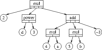
However, doing so results in a rather deeply nested tree which will quickly become inefficient to manipulate. We can improve on this by representing the sum as a sequence of terms, each one being a pair of a purely numeric multiplicative coefficient and its rest. In the same spirit we can store the multiplication as a sequence of terms, each having a numeric exponent and a possibly complicated base, the tree becomes much more flat:
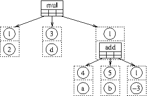
The number 3 above the symbol d shows that mul
objects are treated similarly where the coefficients are interpreted as
exponents now. Addition of sums of terms or multiplication of
products with numerical exponents can be coded to be very efficient with
such a pair-wise representation. Internally, this handling is performed
by most CAS in this way. It typically speeds up manipulations by an
order of magnitude. The overall multiplicative factor 2 and the
additive term -3 look somewhat out of place in this
representation, however, since they are still carrying a trivial
exponent and multiplicative factor 1 respectively. Within GiNaC,
this is avoided by adding a field that carries an overall numeric
coefficient. This results in the realistic picture of internal
representation for
2*d^3*(4*a+5*b-3):
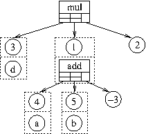
This also allows for a better handling of numeric radicals, since
sqrt(2) can now be carried along calculations. Now it should be
clear, why both classes add and mul are derived from the
same abstract class: the data representation is the same, only the
semantics differs. In the class hierarchy, methods for polynomial
expansion and the like are reimplemented for add and mul,
but the data structure is inherited from expairseq.
Appendix B Package tools 
If you are creating a software package that uses the GiNaC library,
setting the correct command line options for the compiler and linker can
be difficult. The pkgconf utility makes this process
easier. GiNaC supplies all necessary data in ginac.pc (installed
into LIBDIR/pkgconfig by default). To compile a simple
program use 4
g++ -o simple simple.cpp `pkgconf --cflags --libs ginac`
This command line might expand to (for example):
g++ -o simple simple.cpp -lginac -lcln
Not only is the form using pkgconf easier to type, it will
work on any system, no matter how GiNaC was configured.
For packages configured using GNU automake, pkgconf also
provides the PKG_CHECK_MODULES macro to automate the process of
checking for libraries
PKG_CHECK_MODULES(MYAPP, ginac >= MINIMUM_VERSION,
[ACTION-IF-FOUND],
[ACTION-IF-NOT-FOUND])
This macro:
- Determines the location of GiNaC using data from ginac.pc, which is
either found in the default
pkgconfsearch path, or from the environment variablePKG_CONFIG_PATH. - Tests the installed libraries to make sure that their version is later than MINIMUM-VERSION.
- If the required version was found, sets the
MYAPP_CFLAGSvariable to the output ofpkgconf --cflags ginacand theMYAPP_LIBSvariable to the output ofpkgconf --libs ginac, and calls ‘AC_SUBST()’ for these variables so they can be used in generated makefiles, and then executes ACTION-IF-FOUND. - If the required version was not found, executes ACTION-IF-NOT-FOUND.
B.1 Configuring a package that uses GiNaC 
The directory where the GiNaC libraries are installed needs
to be found by your system’s dynamic linkers (both compile- and run-time
ones). See the documentation of your system linker for details. Also
make sure that ginac.pc is in pkgconf’s search path,
See pkgconf.
The short summary below describes how to do this on a GNU/Linux system.
Suppose GiNaC is installed into the directory PREFIX. To tell the linkers where to find the library one should
- edit /etc/ld.so.conf and run
ldconfig. For example,# echo PREFIX/lib >> /etc/ld.so.conf # ldconfig
- or set the environment variables
LD_LIBRARY_PATHandLD_RUN_PATH$ export LD_LIBRARY_PATH=PREFIX/lib $ export LD_RUN_PATH=PREFIX/lib
- or give a ‘-L’ and ‘--rpath’ flags when running configure,
for instance:
$ LDFLAGS='-Wl,-LPREFIX/lib -Wl,--rpath=PREFIX/lib' ./configure
To tell pkgconf where the ginac.pc file is,
set the PKG_CONFIG_PATH environment variable:
$ export PKG_CONFIG_PATH=PREFIX/lib/pkgconfig
Finally, run the configure script
$ ./configure
B.2 Example of a package using GiNaC 
The following shows how to build a simple package using automake and the ‘PKG_CHECK_MODULES’ macro. The program used here is simple.cpp:
#include <iostream>
#include <ginac/ginac.h>
int main()
{
GiNaC::symbol x("x");
GiNaC::ex a = GiNaC::sin(x);
std::cout << "Derivative of " << a
<< " is " << a.diff(x) << std::endl;
return 0;
}
You should first read the introductory portions of the automake manual, if you are not already familiar with it.
Two files are needed, configure.ac, which is used to build the configure script:
dnl Process this file with autoreconf to produce a configure script. AC_INIT([simple], [1.0.0], [simple@example.net]) AC_CONFIG_SRCDIR(simple.cpp) AM_INIT_AUTOMAKE AC_PROG_CXX AC_PROG_INSTALL AC_LANG([C++]) PKG_CHECK_MODULES(SIMPLE, ginac >= 1.8.0) AC_CONFIG_FILES([Makefile]) AC_OUTPUT
The ‘PKG_CHECK_MODULES’ macro does the following: If a GiNaC version greater or equal than 1.8.0 is found, then it defines SIMPLE_CFLAGS and SIMPLE_LIBS. Otherwise, it dies with the error message like
configure: error: Package requirements (ginac >= 1.8.0) were not met: Package dependency requirement 'ginac >= 1.8.0' could not be satisfied. Package 'ginac' has version '1.7.7', required version is '>= 1.8.0' Consider adjusting the PKG_CONFIG_PATH environment variable if you installed software in a non-standard prefix. Alternatively, you may set the environment variables SIMPLE_CFLAGS and SIMPLE_LIBS to avoid the need to call pkg-config. See the pkg-config man page for more details.
And the Makefile.am, which will be used to build the Makefile.
## Process this file with automake to produce Makefile.in bin_PROGRAMS = simple simple_SOURCES = simple.cpp simple_CPPFLAGS = $(SIMPLE_CFLAGS) simple_LDADD = $(SIMPLE_LIBS)
This Makefile.am, says that we are building a single executable, from a single source file simple.cpp. Since every program we are building uses GiNaC we could have simply added SIMPLE_CFLAGS to CPPFLAGS and SIMPLE_LIBS to LIBS. However, it is more flexible to specify libraries and complier options on a per-program basis.
To try this example out, create a new directory and add the three files above to it.
Now execute the following command:
$ autoreconf -i
You now have a package that can be built in the normal fashion
$ ./configure $ make $ make install
Appendix C Bibliography 
- ISO/IEC 14882:2011: Programming Languages: C++
- CLN: A Class Library for Numbers, Bruno Haible
- The C++ Programming Language, Bjarne Stroustrup, 3rd Edition, ISBN 0-201-88954-4, Addison Wesley
- C++ FAQs, Marshall Cline, ISBN 0-201-58958-3, 1995, Addison Wesley
- Algorithms for Computer Algebra, Keith O. Geddes, Stephen R. Czapor, and George Labahn, ISBN 0-7923-9259-0, 1992, Kluwer Academic Publishers, Norwell, Massachusetts
- Computer Algebra: Systems and Algorithms for Algebraic Computation, James H. Davenport, Yvon Siret and Evelyne Tournier, ISBN 0-12-204230-1, 1988, Academic Press, London
- Computer Algebra Systems - A Practical Guide, Michael J. Wester (editor), ISBN 0-471-98353-5, 1999, Wiley, Chichester
- The Art of Computer Programming, Vol 2: Seminumerical Algorithms, Donald E. Knuth, ISBN 0-201-89684-2, 1998, Addison Wesley
- Pi Unleashed, Jörg Arndt and Christoph Haenel, ISBN 3-540-66572-2, 2001, Springer, Heidelberg
- The Role of gamma5 in Dimensional Regularization, Dirk Kreimer, hep-ph/9401354
Concept index 
| Jump to: | A B C D E F G H I K L M N O P Q R S T U V W Z |
|---|
| Index Entry | Section | |
|---|---|---|
| A | ||
abs() | Built-in functions | |
accept() | Visitors and tree traversal | |
| accuracy | Numbers | |
acos() | Built-in functions | |
acosh() | Built-in functions | |
add | Fundamental containers | |
add | Internal representation of products and sums | |
| advocacy | A comparison with other CAS | |
| alternating Euler sum | Multiple polylogarithms | |
antisymmetrize() | Symmetrization | |
append() | Lists | |
archive (class) | Input/output | |
| archiving | Input/output | |
asin() | Built-in functions | |
asinh() | Built-in functions | |
atan() | Built-in functions | |
atanh() | Built-in functions | |
| atom | The class hierarchy | |
| atom | Symbols | |
| Autoconf | Configuration | |
| B | ||
basic_log_kernel() | Iterated integrals | |
bernoulli() | Numbers | |
beta() | Built-in functions | |
binomial() | Built-in functions | |
| branch cut | Built-in functions | |
| building GiNaC | Building GiNaC | |
| C | ||
calchash() | Adding classes | |
canonicalize_clifford() | Non-commutative objects | |
Catalan | Constants | |
| chain rule | Symbolic differentiation | |
charpoly() | Matrices | |
clifford (class) | Non-commutative objects | |
clifford_bar() | Non-commutative objects | |
clifford_inverse() | Non-commutative objects | |
clifford_max_label() | Non-commutative objects | |
clifford_moebius_map() | Non-commutative objects | |
clifford_norm() | Non-commutative objects | |
clifford_prime() | Non-commutative objects | |
clifford_star() | Non-commutative objects | |
clifford_to_lst() | Non-commutative objects | |
clifford_unit() | Non-commutative objects | |
| CLN | Installation | |
| CLN | Numbers | |
coeff() | Polynomial arithmetic | |
collect_common_factors() | Polynomial arithmetic | |
collect() | Polynomial arithmetic | |
color (class) | Non-commutative objects | |
color_d() | Non-commutative objects | |
color_f() | Non-commutative objects | |
color_h() | Non-commutative objects | |
color_ONE() | Non-commutative objects | |
color_T() | Non-commutative objects | |
color_trace() | Non-commutative objects | |
compare_same_type() | Adding classes | |
compare() | Information about expressions | |
| compile_ex | Input/output | |
| compiling expressions | Input/output | |
| complex numbers | Numbers | |
| configuration | Configuration | |
conjugate() | Built-in functions | |
conjugate() | Complex expressions | |
const_iterator | Information about expressions | |
const_postorder_iterator | Information about expressions | |
const_preorder_iterator | Information about expressions | |
constant (class) | Constants | |
| container | The class hierarchy | |
| container | Information about expressions | |
content() | Polynomial arithmetic | |
| contravariant | Indexed objects | |
Converting ex to other classes | Information about expressions | |
| copy-on-write | Expressions are reference counted | |
cos() | Built-in functions | |
cosh() | Built-in functions | |
| covariant | Indexed objects | |
csrc | Input/output | |
csrc_cl_N | Input/output | |
csrc_double | Input/output | |
csrc_float | Input/output | |
| CUBA library | Input/output | |
| D | ||
DECLARE_FUNCTION | Symbolic functions | |
degree() | Polynomial arithmetic | |
delta_tensor() | Indexed objects | |
denom() | Rational expressions | |
| denominator | Rational expressions | |
determinant() | Matrices | |
dflt | Input/output | |
diag_matrix() | Matrices | |
diff() | Symbolic differentiation | |
| differentiation | Symbolic differentiation | |
Digits | Numbers | |
Digits | Numerical evaluation | |
dirac_gamma() | Non-commutative objects | |
dirac_gamma5() | Non-commutative objects | |
dirac_gammaL() | Non-commutative objects | |
dirac_gammaR() | Non-commutative objects | |
dirac_ONE() | Non-commutative objects | |
dirac_slash() | Non-commutative objects | |
dirac_trace() | Non-commutative objects | |
divide() | Polynomial arithmetic | |
doublefactorial() | Numbers | |
| dummy index | Indexed objects | |
| E | ||
Ebar_kernel() | Iterated integrals | |
Eisenstein_h_kernel() | Iterated integrals | |
Eisenstein_kernel() | Iterated integrals | |
ELi_kernel() | Iterated integrals | |
EllipticE() | Built-in functions | |
EllipticK() | Built-in functions | |
epsilon_tensor() | Indexed objects | |
eta() | Built-in functions | |
Euler | Constants | |
| Euler numbers | Symbolic differentiation | |
eval() | Automatic evaluation | |
eval() | Adding classes | |
evalf() | Constants | |
evalf() | Numerical evaluation | |
evalm() | Matrices | |
| evaluation | Automatic evaluation | |
| evaluation | Symbolic functions | |
| evaluation | Adding classes | |
ex_is_equal (class) | Information about expressions | |
ex_is_less (class) | Information about expressions | |
ex_to<…>() | Information about expressions | |
| exceptions | Error handling | |
exp() | Built-in functions | |
| expand trancedent functions | Built-in functions | |
expand_dummy_sum() | Indexed objects | |
expand_options::expand_function_args | Built-in functions | |
expand_options::expand_transcendental | Built-in functions | |
expand() | Indexed objects | |
expand() | Polynomial arithmetic | |
expression (class ex) | Expressions | |
| F | ||
factor() | Polynomial arithmetic | |
factorial() | Built-in functions | |
| factorization | Polynomial arithmetic | |
| factorization | Polynomial arithmetic | |
fibonacci() | Numbers | |
find() | Pattern matching and advanced substitutions | |
| fraction | Numbers | |
| fsolve | What it can do for you | |
| FUNCP_1P | Input/output | |
| FUNCP_2P | Input/output | |
| FUNCP_CUBA | Input/output | |
function (class) | Mathematical functions | |
| G | ||
G() | Built-in functions | |
G() | Built-in functions | |
| Gamma function | Mathematical functions | |
| gamma function | Built-in functions | |
| garbage collection | Expressions are reference counted | |
| GCD | Polynomial arithmetic | |
gcd() | Polynomial arithmetic | |
get_dim() | Indexed objects | |
get_free_indices() | Indexed objects | |
get_metric() | Non-commutative objects | |
get_name() | Symbols | |
get_TeX_name() | Symbols | |
get_value() | Indexed objects | |
| ginac-excompiler | Input/output | |
ginsh | What it can do for you | |
ginsh | Fundamental containers | |
ginsh | What does not belong into GiNaC | |
| GMP | Numbers | |
Gt() | Built-in functions | |
| H | ||
H() | Built-in functions | |
| harmonic polylogarithm | Multiple polylogarithms | |
has() | Expressions | |
has() | Pattern matching and advanced substitutions | |
| Hermite polynomial | How to use it from within C++ | |
| hierarchy of classes | Symbols | |
| hierarchy of classes | Adding classes | |
| history of GiNaC | Introduction | |
hold() | Symbolic functions | |
hold() | Adding classes | |
| hyperbolic function | Mathematical functions | |
| I | ||
I | Numbers | |
| I/O | Input/output | |
idx (class) | Indexed objects | |
imag_part() | Built-in functions | |
imag() | Numbers | |
index_dimensions | Input/output | |
indexed (class) | Indexed objects | |
info() | Information about expressions | |
| input of expressions | Input/output | |
| installation | Installing GiNaC | |
integral (class) | Integrals | |
integration_kernel() | Iterated integrals | |
inverse() (matrix) | Matrices | |
inverse() (numeric) | Numbers | |
iquo() | Numbers | |
irem() | Numbers | |
is_a<…>() | Information about expressions | |
is_equal_same_type() | Adding classes | |
is_equal() | Information about expressions | |
is_exactly_a<…>() | Information about expressions | |
is_polynomial() | Polynomial arithmetic | |
is_zero_matrix() | Matrices | |
is_zero() | Information about expressions | |
isqrt() | Numbers | |
iterated_integral() | Built-in functions | |
iterated_integral() | Built-in functions | |
| iterators | Information about expressions | |
| K | ||
Kronecker_dtau_kernel() | Iterated integrals | |
Kronecker_dz_kernel() | Iterated integrals | |
| L | ||
latex | Input/output | |
| Laurent expansion | Series expansion | |
| LCM | Polynomial arithmetic | |
lcm() | Polynomial arithmetic | |
ldegree() | Polynomial arithmetic | |
let_op() | Structures | |
let_op() | Adding classes | |
lgamma() | Built-in functions | |
Li() | Built-in functions | |
Li2() | Built-in functions | |
| link_ex | Input/output | |
| lists | Lists | |
log() | Built-in functions | |
lorentz_eps() | Indexed objects | |
lorentz_g() | Indexed objects | |
lsolve() | Solving linear systems of equations | |
lst (class) | Lists | |
lst_to_clifford() | Non-commutative objects | |
lst_to_matrix() | Matrices | |
| M | ||
| Machin’s formula | Series expansion | |
map() | Applying a function on subexpressions | |
match() | Pattern matching and advanced substitutions | |
matrix (class) | Matrices | |
metric_tensor() | Indexed objects | |
mod() | Numbers | |
modular_form_kernel() | Iterated integrals | |
| Monte Carlo integration | Input/output | |
mul | Fundamental containers | |
mul | Internal representation of products and sums | |
| multiple polylogarithm | Multiple polylogarithms | |
| multiple zeta value | Multiple polylogarithms | |
multiple_polylog_kernel() | Iterated integrals | |
| N | ||
ncmul (class) | Non-commutative objects | |
| Nielsen’s generalized polylogarithm | Multiple polylogarithms | |
no_index_dimensions | Input/output | |
nops() | Lists | |
nops() | Information about expressions | |
normal() | Rational expressions | |
numer_denom() | Rational expressions | |
numer() | Rational expressions | |
| numerator | Rational expressions | |
numeric (class) | Numbers | |
| O | ||
op() | Lists | |
op() | Information about expressions | |
Order() | Series expansion | |
Order() | Built-in functions | |
| output of expressions | Input/output | |
| P | ||
| pair-wise representation | Internal representation of products and sums | |
| partial fraction decomposition | Polynomial arithmetic | |
| Pattern matching | Pattern matching and advanced substitutions | |
Pi | Constants | |
pkgconf | Package tools | |
pole_error (class) | Error handling | |
| polylogarithm | Multiple polylogarithms | |
| polynomial | Fundamental containers | |
| polynomial | Methods and functions | |
| polynomial division | Polynomial arithmetic | |
| polynomial factorization | Polynomial arithmetic | |
possymbol() | Symbols | |
pow() | Fundamental containers | |
power | Fundamental containers | |
power | Internal representation of products and sums | |
prem() | Polynomial arithmetic | |
prepend() | Lists | |
primpart() | Polynomial arithmetic | |
print_context (class) | Printing | |
print_csrc (class) | Printing | |
print_dflt (class) | Printing | |
print_latex (class) | Printing | |
print_tree (class) | Printing | |
print() | Printing | |
| printing | Input/output | |
| product rule | Symbolic differentiation | |
| product rule | Symbolic functions | |
pseries (class) | Series expansion | |
| pseudo-remainder | Polynomial arithmetic | |
| pseudo-vector | Non-commutative objects | |
psi() | Built-in functions | |
| Q | ||
quo() | Polynomial arithmetic | |
| quotient | Polynomial arithmetic | |
| R | ||
| radical | Internal representation of products and sums | |
rank() | Matrices | |
| rational | Numbers | |
real_part() | Built-in functions | |
real() | Numbers | |
realsymbol() | Symbols | |
reduced_matrix() | Matrices | |
| reference counting | Expressions are reference counted | |
REGISTER_FUNCTION | Symbolic functions | |
relational (class) | Relations | |
relational (class) | Information about expressions | |
rem() | Polynomial arithmetic | |
| remainder | Polynomial arithmetic | |
remove_all() | Lists | |
remove_dirac_ONE() | Non-commutative objects | |
remove_first() | Lists | |
remove_last() | Lists | |
| representation | Internal representation of products and sums | |
| resultant | Polynomial arithmetic | |
resultant() | Polynomial arithmetic | |
return_type_tinfo() | Non-commutative objects | |
return_type_tinfo() | Information about expressions | |
return_type() | Non-commutative objects | |
return_type() | Information about expressions | |
| rounding | Numbers | |
| S | ||
S() | Built-in functions | |
series() | Series expansion | |
| simplification | Rational expressions | |
simplify_indexed() | Indexed objects | |
sin() | Built-in functions | |
sinh() | Built-in functions | |
smod() | Numbers | |
solve() | Matrices | |
spinidx (class) | Indexed objects | |
spinor_metric() | Indexed objects | |
sqrfree_parfrac() | Polynomial arithmetic | |
sqrfree() | Polynomial arithmetic | |
sqrt() | Built-in functions | |
| square-free decomposition | Polynomial arithmetic | |
| square-free partial fraction decomposition | Polynomial arithmetic | |
step() | Built-in functions | |
| STL | Advantages | |
sub_matrix() | Matrices | |
subs() | Symbols | |
subs() | Mathematical functions | |
subs() | Indexed objects | |
subs() | Methods and functions | |
subs() | Substituting expressions | |
subs() | Pattern matching and advanced substitutions | |
sy_anti() | Indexed objects | |
sy_cycl() | Indexed objects | |
sy_none() | Indexed objects | |
sy_symm() | Indexed objects | |
symbol (class) | Symbols | |
symbolic_matrix() | Matrices | |
symmetrize_cyclic() | Symmetrization | |
symmetrize() | Symmetrization | |
symmetry (class) | Indexed objects | |
| T | ||
tan() | Built-in functions | |
tanh() | Built-in functions | |
| Taylor expansion | Series expansion | |
| temporary replacement | Rational expressions | |
tensor (class) | Indexed objects | |
tgamma() | Built-in functions | |
to_cl_N() | Numbers | |
to_double() | Numbers | |
to_int() | Numbers | |
to_long() | Numbers | |
to_polynomial() | Rational expressions | |
to_rational() | Rational expressions | |
trace() | Matrices | |
transpose() | Matrices | |
traverse_postorder() | Visitors and tree traversal | |
traverse_preorder() | Visitors and tree traversal | |
traverse() | Visitors and tree traversal | |
tree | Input/output | |
| tree traversal | Applying a function on subexpressions | |
| tree traversal | Visitors and tree traversal | |
| Tree traversal | Input/output | |
| trigonometric function | Mathematical functions | |
| U | ||
unit_matrix() | Matrices | |
unit() | Polynomial arithmetic | |
unitcontprim() | Polynomial arithmetic | |
| unlink_ex | Input/output | |
user_defined_kernel() | Iterated integrals | |
| V | ||
| variance | Indexed objects | |
varidx (class) | Indexed objects | |
viewgar | Input/output | |
visit() | Visitors and tree traversal | |
visitor (class) | Visitors and tree traversal | |
| W | ||
wildcard (class) | Pattern matching and advanced substitutions | |
| Z | ||
| Zeta function | What it can do for you | |
zeta() | Built-in functions | |
zeta() | Built-in functions | |
| Jump to: | A B C D E F G H I K L M N O P Q R S T U V W Z |
|---|